Introduction

lbh15 (Lead Bismuth Handbook 2015) is a Python package that implements the thermo-physical and the thermo-chemical properties of lead, bismuth and lead-bismuth eutectic (lbe) metal alloy available from the handbook edited by OECD/NEA [1]: https://www.oecd-nea.org/jcms/pl_14972/handbook-on-lead-bismuth-eutectic-alloy-and-lead-properties-materials-compatibility-thermal-hydraulics-and-technologies-2015-edition.

lbh15 offers a standard implementation for use of these properties in scientific applications. In particular, this package is used for numerical simulation and experimental activities supporting the development of nuclear reactors that employ heavy liquid metals as primary coolant.

The thermo-physical properties implemented in the package are listed in Table 1.

Table 1 *lbh15* thermo-physical properties from the handbook edited by OECD/NEA.
Property	Symbol	Units
Melting temperature	\(T_{m0}\)	\([K]\)
Melting latent heat	\(Q_{m0}\)	\([J/kg]\)
Boiling temperature	\(T_{b0}\)	\([K]\)
Vaporization heat	\(Q_{b0}\)	\([J/kg]\)
Saturation vapor pressure	\(p_s\)	\([Pa]\)
Surface tension	\(\sigma\)	\([N/m]\)
Density	\(\rho\)	\([kg/m^3]\)
Thermal expansion coefficient	\(\alpha\)	\([1/K]\)
Speed of sound	\(u_s\)	\([m/s]\)
Isentropic compressibility	\(\beta_s\)	\([1/Pa]\)
Mass-specific heat capacity	\(c_p\)	\([J/(kg{\cdot}K)]\)
Mass-specific enthalpy	\(h\)	\([J/kg]\)
Dynamic viscosity	\(\mu\)	\([Pa{\cdot}s]\)
Electrical resistivity	\(r\)	\([{\Omega}{\cdot}m]\)
Thermal conductivity	\(k\)	\([W/(m{\cdot}K)]\)

The dimensionless Prandtl number (\(Pr\)) can be queried as instance attribute as well.

The thermo-chemical properties implemented since version 1.2.0 are listed in Table 2 (basic properties), Table 3 (solubilities, diffusivities and Oxygen partial pressure), Table 4 (lower limits of oxygen concentration for oxide layers generation when the corresponding metal is considered at its saturation concentration) and Table 5 (lower limits of oxygen concentration for oxide layers generation multiplied by the corresponding metal concentration raised to a specific coefficient).

Table 2 *lbh15* thermo-chemical properties from the handbook edited by OECD/NEA: basic data.
Property	Symbol	Units	Lead	LBE	Bismuth
Molar-specific enthalpy	\(H\)	\([J/mol]\)	✔	✔	✔
Molar-specific entropy	\(S\)	\([J/(mol \cdot K)]\)	✔	✔	✔
Gibbs free energy	\(G\)	\([J/mol]\)	✔	✔	✔

Table 3 *lbh15* thermo-chemical properties from the handbook edited by OECD/NEA: solubilities, diffusivities and oxygen partial pressure.
Property	Symbol	Units	Lead	LBE	Bismuth
Iron solubility	\(S_{\ce{Fe}}\)	\([wt.\%]\)	✔	✔	✔
Nickel solubility	\(S_{\ce{Ni}}\)	\([wt.\%]\)	✔	✔	✔
Chromium solubility	\(S_{\ce{Cr}}\)	\([wt.\%]\)	✔	✔	✔
Silicon solubility	\(S_{\ce{Si}}\)	\([wt.\%]\)	✔	\(-\)	\(-\)
Oxygen solubility	\(S_{\ce{O}}\)	\([wt.\%]\)	✔	✔	✔
Oxygen diffusivity	\(D_{\ce{O}}\)	\([cm^2/s]\)	✔	✔	✔
Iron diffusivity	\(D_{\ce{Fe}}\)	\([cm^2/s]\)	✔	✔	\(-\)
Cobalt diffusivity	\(D_{\ce{Co}}\)	\([cm^2/s]\)	✔	\(-\)	\(-\)
Selenium diffusivity	\(D_{\ce{Se}}\)	\([cm^2/s]\)	✔	\(-\)	\(-\)
Indium diffusivity	\(D_{\ce{In}}\)	\([cm^2/s]\)	✔	\(-\)	\(-\)
Tellurium diffusivity	\(D_{\ce{Tl}}\)	\([cm^2/s]\)	✔	\(-\)	\(-\)
Oxygen partial pressure divided by the oxygen concentration squared	\(P_{\ce{O2}}\)	\([atm/wt.\%^2]\)	✔	✔	✔

Table 4 *lbh15* thermo-chemical properties from the handbook edited by OECD/NEA: lower limits of oxygen concentration for oxide layers generation when the corresponding metal is considered at its saturation concentration.
Property	Symbol	Units	Lead	LBE	Bismuth
\(\ce{Fe3O4}\)-related lower limit of \(\ce{O2}\) concentration in case of \(\ce{Fe}\)-saturated metal	\(C_{\ce{O2}, \ce{Fe}(sat)}\)	\([wt.\%]\)	✔	✔	\(-\)
\(\ce{NiO}\)-related lower limit of \(\ce{O2}\) concentration in case of \(\ce{Ni}\)-saturated metal	\(C_{\ce{O2}, \ce{Ni}(sat)}\)	\([wt.\%]\)	✔	✔	\(-\)
\(\ce{Cr2O3}\)-related lower limit of \(\ce{O2}\) concentration in case of \(\ce{Cr}\)-saturated metal	\(C_{\ce{O2}, \ce{Cr}(sat)}\)	\([wt.\%]\)	✔	✔	\(-\)
\(\ce{SiO2}\)-related lower limit of \(\ce{O2}\) concentration in case of \(\ce{Si}\)-saturated metal	\(C_{\ce{O2}, \ce{Si}(sat)}\)	\([wt.\%]\)	✔	✔	\(-\)
\(\ce{Al2O3}\)-related lower limit of \(\ce{O2}\) concentration in case of \(\ce{Al}\)-saturated metal	\(C_{\ce{O2}, \ce{Al}(sat)}\)	\([wt.\%]\)	✔	✔	\(-\)

Table 5 *lbh15* thermo-chemical properties from the handbook edited by OECD/NEA: lower limits of oxygen concentration for oxide layers generation multiplied by the corresponding metal concentration raised to a specific coefficient.
Property	Symbol	Units	Lead	LBE	Bismuth
Lead chemical activity in LBE	\(\alpha_{\ce{Pb}}\)	\([-]\)	\(-\)	✔	\(-\)
Bismuth chemical activity in LBE	\(\alpha_{\ce{Bi}}\)	\([-]\)	\(-\)	✔	\(-\)
\(\ce{Fe3O4}\)-related lower limit of \(\ce{O2}\) concentration times \(\ce{Fe}\) concentration raised to 3/4	\(C_{\ce{O2}} \cdot C_{\ce{Fe}}^{3/4}\)	\([wt.\%]\)	✔	✔	\(-\)
\(\ce{NiO}\)-related lower limit of \(\ce{O2}\) concentration times \(\ce{Ni}\) concentration	\(C_{\ce{O2}} \cdot C_{\ce{Ni}}\)	\([wt.\%]\)	✔	✔	\(-\)
\(\ce{Cr2O3}\)-related lower limit of \(\ce{O2}\) concentration times \(\ce{Cr}\) concentration raised to 2/3	\(C_{\ce{O2}} \cdot C_{\ce{Cr}}^{2/3}\)	\([wt.\%]\)	✔	✔	\(-\)
\(\ce{SiO2}\)-related lower limit of \(\ce{O2}\) concentration times \(\ce{Si}\) concentration raised to 1/2	\(C_{\ce{O2}} \cdot C_{\ce{Si}}^{1/2}\)	\([wt.\%]\)	✔	\(-\)	\(-\)

The pressure at which to evaluate the properties can be specified at object’s instantiation. Otherwise, all the properties are given at atmospheric pressure (\(101325\) \([Pa]\)) by default. The correlations’ validity range is checked at evaluation in terms of temperature value, raising a warning in case it is not satisfied (see Basic Usage section for more details). Some examples of instantiation are provided using also a target property value, see Initialization from Properties (experimental) section for instance. For the sake of completeness, the correlations are also reported in the docstring documentation. The implementation is fully object-oriented to guarantee easy maintainability, extension and customization of the package (see Advanced Usage section).

Go to API Guide section to see the full code documentation.

lbh15 is developed and maintained by the Codes & Methods group of newcleo (https://www.newcleo.com/) and is released under the GNU Lesser General Public License 3 (see License section).

lbh15 is listed among the Open-source Nuclear Codes for Reactor Analysis (https://nucleus.iaea.org/sites/oncore/SitePages/List%20of%20Codes.aspx) by IAEA.

Project Structure

The project is organized according to the following folder structure:

<lbh15 parent folder>
  ├── docs/
  ├── lbh15/
  ├── tests/
  ├── tutorials/
  ├── CHANGELOG.rst
  ├── LICENSE
  ├── MANIFEST.in
  ├── README.rst
  ├── pyproject.toml
  └── setup.py

lbh15: contains all modules, classes and methods implemented in lbh15;
docs: contains files for the generation of the documentation by Sphinx;
tests: collection of tests used to verify the correct implementation;
tutorials: collection of tutorials and examples, each one into a dedicated sub-folder.

Dependencies

To run the code, the following dependencies must be satisfied:

Python \(>= 3.8.10\)
SciPy \(>= 1.8.1\)
NumPy \(>= 1.22.3\)

To build the documentation in both html and LaTeX formats, the following dependencies must be satisfied:

sphinx \(>= 6.2.1\)
sphinx-rtd-theme \(>= 1.3.0\)
myst-parser \(>= 1.0.0\)
sphinxcontrib-bibtex \(>= 2.5.0\)

Installation

To install the lbh15 package, please type the following command:

pip install lbh15

Otherwise, clone the package from https://github.com/newcleo-dev-team/lbh15.git and execute the following command inside the resulting folder:

pip install .

To upgrade the lbh15 package, please type the install command along with the --upgrade or -U flag:

pip install --upgrade lbh15

The Sphinx documentation can be built in html and LaTeX by executing the following commands, respectively, in the docs/ folder:

make html

make latexpdf

The html documentation is available on GitHub Pages at https://newcleo-dev-team.github.io/lbh15/index.html.

To see the available templates for generating the documentation in PDF format and to choose among them, please look at the docs/conf.py file.

Getting Started

This section contains some examples of basic usage and possible customization of the lbh15 package. More examples are available in Lead, Bismuth and LBE classes.

Basic Usage

This section shows a few examples of basic usage of lbh15.

Create a Lead instance using Celsius degrees as temperature unit and print the corresponding dynamic viscosity mu:

>>> from scipy.constants import convert_temperature
>>> from lbh15 import Lead
>>> # Initialize Lead object with T=395 Celsius
>>> liquid_lead = Lead(T=convert_temperature(395.0, 'C', 'K'))
>>> # Print lead dynamic viscosity in [Pa*s]
>>> liquid_lead.mu
0.0022534948395446985

Create two instances of Lead class, one at atmospheric pressure and one at twenty times the atmospheric pressure. Then compare their density values rho:

>>> from lbh15 import Lead
>>> from scipy.constants import atm
>>> # Initialize first object, default pressure is atm
>>> liquid_lead = Lead(T=800)
>>> # Initialize the second object by specifying the pressure
>>> liquid_lead_2 = Lead(T=800, p=20*atm)
>>> # Compare their density
>>> liquid_lead.rho, liquid_lead_2.rho
(10417.4, 10418.185181757714)

Create an instance of Lead class at a given temperature T, then change the temperature value. Compare the conductivity values k at the two temperatures:

>>> from lbh15 import Lead
>>> liquid_lead = Lead(T=750)
>>> liquid_lead.k
17.45
>>> liquid_lead.T = 1200
>>> liquid_lead.k
22.4

Create an instance of Lead class at a given temperature T, then change the temperature value. Compare the oxygen diffusivity values o_dif at the two temperatures:

>>> from lbh15 import Lead
>>> liquid_lead = Lead(T=700)
>>> liquid_lead.o_dif
4.11000872874867e-06
>>> liquid_lead.T = 850
>>> liquid_lead.o_dif
6.708316471487037e-06

Request a property outside the range of validity of the corresponding correlation. In this example, a Lead object is initialized using a temperature value T that is outside the range of physical validity of the surface tension sigma correlation:

>>> from lbh15 import Lead
>>> liquid_lead = Lead(T=1400.0)
>>> liquid_lead.sigma
<stdin>:1: UserWarning: The surface tension is requested at temperature value of 1400.00 K that is not in validity range [600.60, 1300.00] K
0.3676999999999999

Get summary information of the liquid metal using the overriden __repr__ dunder method (the warnings about out-of-range correlations are also written):

>>> from lbh15 import Lead
>>> liquid_lead = Lead(T=900)
>>> liquid_lead
.local/lib/python3.9/site-packages/lbh15/_lbh15.py:740: UserWarning: The iron diffusivity is requested at temperature value of 900.00 K that is not in validity range [973.00, 1273.00] K
  attr_value = getattr(self, key)
.local/lib/python3.9/site-packages/lbh15/_lbh15.py:740: UserWarning: The silicon solubility is requested at temperature value of 900.00 K that is not in validity range [1323.00, 1523.00] K
  attr_value = getattr(self, key)
.local/lib/python3.9/site-packages/lbh15/_lbh15.py:740: UserWarning: The cobalt diffusivity is requested at temperature value of 900.00 K that is not in validity range [1023.00, 1273.00] K
  attr_value = getattr(self, key)
Lead(T=900.00, p=101325.00, fe_sol=2.02e-04, lim_cr=1.52e-15, in_dif=4.91e-05, lim_si_sat=2.69e-17, fe_dif=1.38e-05, k=19.10, lim_fe_sat=1.60e-07, lim_fe=2.71e-10, beta_s=3.24e-11, se_dif=6.02e-05, H=9010.76, lim_ni_sat=9.30e-05, r=1.09e-06, si_sol=8.10e-05, lim_ni=6.01e-05, alpha=1.24e-04, h=43488.20, cp=142.52, p_s=0.12, lim_si=2.42e-19, G=-1.96e+03, co_dif=2.38e-05, o_pp=4.23e-11, lim_cr_sat=4.92e-13, o_dif=7.62e-06, rho=10289.45, ni_sol=0.65, S=12.19, te_dif=3.71e-05, lim_al_sat=1.54e-22, cr_sol=1.71e-04, o_sol=4.23e-03, u_s=1731.60, mu=1.49e-03, sigma=0.42)

Initialization from Properties (experimental)

The lbh15 package gives the possibility to instantiate a liquid metal object by simply knowing the value of one of its properties (see Lead, Bismuth and LBE classes documentation for the full list). This is accomplished by finding the root of the correlation function matching the target property value. Such function, which is a physical property correlation, must be injective in the range considered for the root. Note that this is a necessary, but not jointly sufficient condition to find a root for the function.

Since the existence of a (single) root cannot be guaranteed for every correlation, this functionality is marked as experimental: the user is invited to double-check the result (see Advanced Usage section).

In the following, some examples are provided:

Initialize an LBE instance, i.e., lead-bismuth-eutectic object, by setting its density rho and retrieve the corresponding temperature T in Kelvin degrees:

>>> from lbh15 import LBE
>>> # Initialize LBE with rho=9800 [kg/m^3]
>>> liquid_lbe = LBE(rho=9800)
>>> # Print lbe temperature in [K]
>>> liquid_lbe.T
978.3449342614074

Compare properties of different liquid metal objects at a given temperature. In this example, a Lead object is initialized by specifying a value of the thermal conductivity k; then, a Bismuth object is initialized using the Lead instance temperature T in Kelvin degrees. Finally, the thermal conductivity k of the Bismuth object is printed for comparison purposes:
```
>>> from lbh15 import Lead
>>> from lbh15 import Bismuth
>>> # Inititialize lead with k=17.37 [W/(m*K)]
>>> liquid_lead = Lead(k=17.37)
>>> # Initialize bismuth with lead temperature in K
>>> liquid_bismuth = Bismuth(T=liquid_lead.T)
>>> # Print bismuth conductivity
>>> liquid_bismuth.k
14.395909090909091
```

The initialization from mass-specific heat capacity \(c_p\) needs some attention because the corresponding function of temperature is not injective. In particular, two temperature values may be possible for the same value of \(c_p\). This occurrence must be handled carefully. Currently, the package allows the user to look for the root in the two distinct ranges where the function is monotone. The default range index is 0, which corresponds to the lowest temperature range. Here is an example with Lead class (the same holds for Bismuth and LBE classes):

>>> from lbh15 import Lead
>>> from lbh15 import lead_properties
>>> # Get an instance of cp property, sobolev2011 correlation
>>> cp = lead_properties.cp_sobolev2011()
>>> # Compute correlation bounds (min, max, T_at_min, T_at_max)
>>> cp.compute_bounds()
>>> # Visualize temperature in [K] corresponding to cp min
>>> cp.T_at_min
1568.6647571773037
>>> # Visualize minimum value of cp in [J/(kg*K)]
>>> cp.min
136.34864915749822
>>> # Initialize first object with default index
>>> lead_cp_1 = Lead(cp=136.6)
>>> # Change default cp index for selecting second root, root_index=1
>>> Lead.set_root_to_use('cp', root_index=1)
>>> # Initialize second object
>>> lead_cp_2 = Lead(cp=136.6)
>>> # Print their temperatures in [K]
>>> lead_cp_1.T, lead_cp_2.T
(1437.4148683656551, 1699.157333532332)

Advanced Usage

Advanced usage includes the possibility of adding new properties and new correlations. First of all, the user should be aware of the properties that are currently available along with the correlations. The method Lead.available_correlations() provides this information for a Lead instance (the same goes for Bismuth and LBE instances). Two examples of use are provided, the first one asking for the available correlations for all the implemented properties, the second one asking for the available correlations for a few specific properties, that is, the heat capacity and the speed of sound:

>>> from lbh15 import Lead
>>> Lead.available_correlations()
defaultdict(<class 'list'>, {'k': ['lbh15'], 'lim_ni': ['lbh15'], 'u_s': ['sobolev2011'], 'mu': ['lbh15'], 'H': ['lbh15'], 'lim_cr': ['venkatraman1988', 'alden1958', 'gosse2014'], 'sigma': ['jauch1986'], 'cp': ['sobolev2011', 'gurvich1991'], 'cr_sol': ['venkatraman1988', 'gosse2014', 'alden1958'], 'in_dif': ['lbh15'], 'o_pp': ['taskinen1979', 'charle1976', 'alcock1964', 'otsuka1979', 'otsuka1981', 'fisher1966', 'isecke1977', 'szwarc1972', 'ganesan2006'], 'lim_cr_sat': ['lbh15'], 'si_sol': ['lbh15'], 'fe_dif': ['lbh15'], 'lim_si': ['lbh15'], 'o_dif': ['charle1976', 'swzarc1972', 'arcella1968', 'gromov1996', 'ganesan2006b', 'otsuka1975', 'homna1971'], 'G': ['lbh15'], 'p_s': ['sobolev2011'], 'beta_s': ['lbh15'], 'se_dif': ['lbh15'], 'lim_al_sat': ['lbh15'], 'ni_sol': ['gosse2014'], 'r': ['lbh15'], 'S': ['lbh15'], 'h': ['sobolev2011'], 'alpha': ['lbh15'], 'co_dif': ['lbh15'], 'lim_si_sat': ['lbh15'], 'lim_fe_sat': ['lbh15'], 'fe_sol': ['gosse2014'], 'lim_fe': ['lbh15'], 'rho': ['sobolev2008a'], 'te_dif': ['lbh15'], 'lim_ni_sat': ['lbh15'], 'o_sol': ['lbh15']})
>>> Lead.available_correlations(["cp", "u_s"])
{'cp': ['gurvich1991', 'sobolev2011'], 'u_s': ['sobolev2011']}

In the first example, the keys of the returned dictionary represents all the properties currently available, and, for each one, a list is provided containing the names of all the related correlations. The generic name lbh15 is used in case the correlation’s name is not specified in the reference handbook [1]. In the second example, the structure of the returned dictionary is the same, but containing only data for the required properties.

The rest of this chapter is divided into two sections, the first describing how to add a new correlation to an existing property, the second describing how to add a new property with its correlation.

How to Add New Correlations

This section shows how to define a custom correlation for the density of liquid lead that does not depend on pressure, and how to use it instead of the default one (the same holds for Bismuth and LBE classes).

Let’s implement the new property in <execution_dir>/custom_properties/lead_properties.py as:

from scipy.constants import atm
from lbh15.properties.interface import PropertyInterface
from lbh15.properties.interface import range_warning

class rho_custom_corr(PropertyInterface):
    @range_warning
    def correlation(self, T, p=atm, verbose=False):
        "Implement here the user-defined correlation."
        return 11400 - 1.2*T

    @property
    def range(self):
        return [700.0, 1900.0]

    @property
    def units(self):
        return "[kg/m^3]"

    @property
    def name(self):
        return "rho"

    @property
    def long_name(self):
        return "custom density"

    @property
    def description(self):
        return "Liquid lead " + self.long_name

    @property
    def correlation_name(self):
        return "custom2022"

Note

It is mandatory to override the correlation method and the range, units, long_name and description properties.

Note

Properties are not allowed having the name starting with __. This means that neither the name of the corresponding class nor the name provided by the name attribute must start with __.

Note

It is strongly recommended to use the @range_warning decorator so that the correlation range is checked when property is queried as liquid metal property and warning is printed, if any, as in Basic Usage section.

Then, provided that the execution is performed in <execution_dir>, one can check the correct implementation as follows:

>>> from lbh15 import Lead
>>> import os
>>> Lead.set_custom_properties_path(os.getcwd() + '/custom_properties/lead_properties.py')
>>> Lead.available_correlations("rho")
{'rho': ['sobolev2008a', 'custom2022']}

The correlations available for the density property rho are now 2: sobolev2008a and custom2022. If the density correlation is not specified for a new object instantiation, the last one in the list will be selected by default:

>>> liquid_lead = Lead(T=1000)
>>> liquid_lead.rho_info()
rho:
      Value: 10200.00 [kg/m^3]
      Validity range: [700.00, 1900.00] K
      Correlation name: 'custom2022'
      Long name: custom density
      Units: [kg/m^3]
      Description:
              Liquid Lead custom density

Once introduced the new correlation custom2022 for the density rho, the user can choose which one to use by means of the method Lead.set_correlation_to_use(), according to the following example:

>>> # Use default one
>>> Lead.set_correlation_to_use('rho', 'sobolev2008a')
>>> # Get an instance of lead object at T=1000 K
>>> liquid_lead_1 = Lead(T=1000)
>>> # Print info about rho
>>> liquid_lead_1.rho_info()
rho:
      Value: 10161.50 [kg/m^3]
      Validity range: [600.60, 2021.00] K
      Correlation name: 'sobolev2008a'
      Long name: density
      Units: [kg/m^3]
      Description:
              Liquid lead density
>>> # Use the custom implementation of density
>>> Lead.set_correlation_to_use('rho', 'custom2022')
>>> # Get another instance of lead object with new rho
>>> liquid_lead_2 = Lead(T=1000)
>>> # Compare the density of the two objects
>>> liquid_lead_1.rho, liquid_lead_2.rho
(10161.5 10200.0)
>>> # Print full info about density of second instance
>>> liquid_lead_2.rho_info()
rho:
      Value: 10200.00 [kg/m^3]
      Validity range: [700.00, 1900.00] K
      Correlation name: 'custom2022'
      Long name: custom density
      Units: [kg/m^3]
      Description:
              Liquid Lead custom density

It is also possible to change the correlation used by a liquid metal object instance by calling the Lead.change_correlation_to_use() method on the instance itself.

How to Add New Properties

This section describes how to add new properties to the liquid metal objects. For instance, let’s implement in <execution_dir>/custom_properties/double_T.py the custom property double_T that is simply the double of the temperature:

from scipy.constants import atm
from lbh15.properties.interface import PropertyInterface
from lbh15.properties.interface import range_warning

class T_double(PropertyInterface):
    @range_warning
    def correlation(self, T, p=atm, verbose=False):
        "Return the temperature value multiplied by 2."
        return 2*T

    @property
    def range(self):
        return [700.0, 1900.0]

    @property
    def units(self):
        return "[K]"

    @property
    def name(self):
        return "T_double"

    @property
    def long_name(self):
        return "double of the temperature"

    @property
    def description(self):
        return "Liquid lead " + self.long_name

    @property
    def correlation_name(self):
        return "double2022"

The new custom property can be set as Lead attribute by specifying the path to the module where it is defined:

>>> from lbh15 import Lead
>>> import os
>>> Lead.set_custom_properties_path(os.getcwd() + '/custom_properties/lead_properties.py')
>>> # Initialization of lead object at T=750 K
>>> liquid_lead = Lead(T=750)
>>> # Get T_double
>>> liquid_lead.T_double
1500
>>> # Get its info
>>> liquid_lead.T_double_info()
T_double:
        Value: 1500.00 [K]
        Validity range: [700.00, 1900.00] K
        Correlation name: 'double2022'
        Long name: double of the temperature
        Units: [K]
        Description:
                Liquid lead double of the temperature

Each new property implemented by the user is also available at initialization.

Note

The paths of the modules to load the properties from must be absolute.

Learn More

This section contains additional information about the chemistry of heavy liquid metals in presence of dispersed oxygen in the bulk. It is made of two parts. The first part, presented in Oxygen Control section, describes the oxygen-related correlations implemented in lbh15 and how they have been obtained. The second part, presented in Tutorials section, describes a tutorial application delivered with lbh15, which is a representation of a simple oxygen control system applied to a liquid lead volume.

Oxygen Control

In lead and lbe systems, oxygen is the most important chemical element, which results from start-up operations, maintenance services and, possibly, incidental contaminations ([1]). To operate a nuclear reactor cooled by a lead alloy, it is thus important to determine the upper and the lower oxygen concentration limits.

Oxygen Concentration Upper Limit

The upper limit corresponds to the oxygen concentration value above which contamination by coolant oxides occurs. It is represented by the oxygen solubility in lead and lbe alloys. lbh15 provides these properties in the lead_thermochemical_properties.solubility_in_lead and lbe_thermochemical_properties.solubility_in_lbe modules. The implemented data are extracted from [1], table 3.5.2, “Oxygen solubility in liquid Pb, Bi and LBE”, page 157: they were obtained by linear regression of several correlations specified therein.

Oxygen Concentration Lower Limit

The lower limit corresponds to the minimum value of the oxygen concentration enabling the formation of a protective oxide layer on the structural material. The oxide layer formation is possible only when the oxygen potential in the liquid metal is above the potential leading to the protective film formation. The correlations implemented in the lead_thermochemical_properties.lead_oxygen_limits and lbe_thermochemical_properties.lbe_oxygen_limits modules for computing the lower limits of oxygen concentration are obtained by applying the methodology described in [1], chapter 4, part 4.2.2, pages 187-192. A brief summary is provided in the following.

First of all, the reference reaction equation and the associated Gibbs free energy are determined. Then, the oxygen concentration is expressed as a function of temperature. Eventually, two kinds of correlations, based on two different assumptions, are derived.

The equation (3) of the oxidation reaction is set by considering that it occurs between the metal and the oxygen, with the oxygen supposed in solution as dissolved \(\ce{PbO}\) below its saturation limit. The formation equation (1) of the metal oxide (equation 4.5, page 188 of [1]) is combined with the formation equation (2) of \(\ce{PbO}\), (table 4.2.2, page 189 of [1]):

(1)\[\ce{\frac{2X}{Y}Me_{\left(dissolved\right)} + O_{2\left(dissolved\right)} -> \frac{2}{Y}Me_XO_Y}\]

(2)\[\ce{2Pb + O_2 -> 2PbO}\]

thus resulting in the following oxidation reaction equation for a mole of \(\ce{PbO}\):

(3)\[\ce{\frac{X}{Y}Me_{\left( dissolved \right)} + O_{\left(dissolved\right)} + PbO -> \frac{1}{Y}Me_XO_Y + Pb + O}\]

where:

\(\ce{Me}\) represents the metal of the structural material involved in the oxidation reaction,

\(\ce{X}\) and \(\ce{Y}\) are coefficients specific to the reaction.

The Gibbs free energy associated to equation (3) is:

\[ \begin{align}\begin{aligned}\Delta G^0_{\left(3\right)} & = \frac{\Delta G^0_{\left(1\right)}-\Delta G^0_{\left(2\right)}}{2}\\& = \frac{\left(\Delta H^0_{\left(1\right)}-T\cdot\Delta S^0_{\left(1\right)}\right)-\left(\Delta H^0_{\left(2\right)}-T\cdot\Delta S^0_{\left(2\right)}\right)}{2}\\& = \frac{\Delta H^0_{\left(3\right)}-T\cdot\Delta S^0_{\left(3\right)}}{2},\end{aligned}\end{align} \]

where:

\(\Delta G^0_{\left(i\right)}\) is the Gibbs free energy of formation related to the (\(i\))-th reaction equation;

\(\Delta H^0_{\left(3\right)} = \Delta H^0_{\left(1\right)}-\Delta H^0_{\left(2\right)}\) is the formation enthalpy related to equation (3);

\(\Delta S^0_{\left(3\right)} =\Delta S^0_{\left(1\right)}-\Delta S^0_{\left(2\right)}\) is the formation entropy related to equation (3);

\(\Delta H^0\) and \(\Delta S^0\) values for each reaction are taken from the table 4.2.2 of [1].

In general, the Gibbs free energy of a reaction can also be expressed in the following way:

\[\Delta_rG^0 \left(T\right) = -R \cdot T \cdot \ln{\left(K \left(T\right)\right)},\]

where:

\(T\) is the temperature in \(\left[K\right]\);

\(R\) is the molar gas constant in \(\left[J\cdot K^{-1} \cdot mol^{-1}\right]\);

\(\Delta_rG^0 \left(T\right)\) is the standard free enthalpy of reaction at constant pressure and temperature in \(\left[J\cdot mol^{-1}\right]\);

\(K \left(T\right) = \prod\limits_{i=1}^{N} \alpha_i^{\nu_i}\) is the equilibrium constant, being \(\alpha_i\) the chemical activity of the \(i\)-th species at the equilibrium, \(\nu_i\) the stoichiometric coefficient of the \(i\)-th species in the related reaction (positive for the reaction products and negative for the reactants), and \(N\) the number of components appearing in the related reaction.

In detail, the chemical activity \(\alpha\) is a dimensionless quantity used to express the deviation of a mixture of chemical substances from a standard behavior. It is defined by the following relations:

\(\alpha_i = \gamma_i\cdot\chi_i\) , being \(\gamma\) the dimensionless activity coefficient of the \(i\)-th species and \(\chi_i\) the molar fraction of the same species;

\(\alpha_i = \gamma_i\cdot\frac{C_i}{C_{iref}}\), being \(C_i\) the concentration of the \(i\)-th species in the mixture and \(C_{iref}\) the reference concentration for the same species.

In [1], the concentration at saturation is adopted as reference concentration. In addition, by definition, the activity coefficient is assumed equal to one in two cases: when the related species is a pure chemical element, and when it is very diluted. The activity of a pure element can then be defined as:

\[\alpha_i=C_i / C_i^{sat}.\]

About the chemical activity of lead in lbe, lbh15 implements the correlation proposed by Gossé (2014) and written in chapter 3.3, part 3.3 of [1].

The aim is now to develop, for each possible dissolved metal, a correlation for the lower limit of the oxygen concentration that has the same structure as the equation 4.12, part 4.2.2 of [1]. Starting from the oxidation reaction equation (3), the following substitution is applied:

\[\Delta_rG^0 \left( T \right) = -RT\ln{ \left( \frac{\alpha_{\ce{Pb}} \cdot \alpha_{\ce{Me_XO_Y}}^{\frac{1}{Y}}}{\alpha_{\ce{PbO}}\cdot\alpha_{\ce{Me_{\left( dissolved \right)}}}^{\frac{X}{Y}}} \right)},\]

where the term \(\alpha_{\ce{Me_XO_Y}}\) can be considered equal to one: the lower limit is to be found of the oxygen concentration, thus the metal oxide is considered very diluted.

By considering the oxygen dissolved in the solution in the form of \(\ce{PbO}\) below its saturation limit, as stated in [1], thus taking the chemical activity of the dissolved oxygen equal to the chemical activity of the dissolved \(\ce{PbO}\), and by applying some transformations, one can obtain:

(4)\[\ln{\left( C_{\ce{O}} \right)} = \frac{X}{Y} \cdot \ln{\left(\frac{C_{\ce{Me}}^{sat}}{C_{\ce{Me}}}\right)} + \frac{\Delta H^0_{\left(3\right)}}{2RT} - \frac{\Delta S^0_{\left(3\right)}}{2R} + \ln{\left(\alpha_{\ce{Pb}} \cdot C_{\ce{O}}^{sat}\right)}.\]

In the above equation, the unknows are two, that is, the oxygen concentration \(C_{\ce{O}}\) and the concentration \(C_{\ce{Me}}\) of the dissolved metal, thus preventing the direct computation of the solution. For achieving a useful correlation, the user can choose between two strategies that are proposed and adopted in lbh15. They differ on how they treat the chemical activity of the dissolved metal. The actual activities at the interface are influenced by how diffusion, convection and mass transfer phenomena interact in the liquid metal boundary layer. In spite of the ongoing research, the exact values for the chemical activities of the dissolved metal and of the oxygen are not known.

The first approach is to consider the chemical activity of the dissolved metal equal to one. In this way, the first and the second terms of the right hand side of equation (4) become zero, enabling to compute the lower limit of the oxygen concentration directly through the following relation:

\[C_{\ce{O}} = \alpha_{\ce{Pb}} \cdot C_{\ce{O}}^{sat} \cdot \exp{\left(\frac{\Delta H^0_{\left(3\right)}}{2RT} - \frac{\Delta S^0_{\left(3\right)}}{2R} \right)},\]

where:

\(\Delta H^0_{\left(3\right)}\) and \(\Delta S^0_{\left(3\right)}\) are extracted from table 4.2.2 of [1];

\(C_{\ce{O}}^{sat}\) is computed by adopting the recommended coefficients from table 3.5.2 of [1];

\(\alpha_{\ce{Pb}}\) is taken equal to one in pure Lead, while in lbe it is computed by adopting the correlation proposed by Gossé as indicated at page 146 of [1].

The second approach does not exploit any assumption. In order to make equation (4) solvable, the two unknowns \(C_{\ce{O}}^{sat}\) and \(C_{\ce{Me}}\) are collected into one single unknown, thus expressing equation (4) in terms of \(C_{\ce{O}} \cdot C_{\ce{Me}}^{\frac{X}{Y}}\), as indicated in the following:

\[C_{\ce{O}} \cdot C_{\ce{Me}}^{\frac{X}{Y}} = \alpha_{\ce{Pb}} \cdot C_{\ce{O}}^{sat} \cdot \left(C_{\ce{Me}}^{sat}\right)^{X/Y} \cdot \exp{\left(\frac{\Delta H^0_{\left(3\right)}}{2RT} - \frac{\Delta S^0_{\left(3\right)}}{2R}\right)},\]

where:

\(C_{\ce{Me}}^{sat}\) values are computed by using the data from table 3.5.1 of [1];

\(\Delta H^0_{\left(3\right)}\), \(\Delta S^0_{\left(3\right)}\), \(C_{\ce{O}}^{sat}\) and \(\alpha_{\ce{Pb}}\) are computed as already indicated for the approach described above.

Ranges of Validity

As stated in the previous section, multiple correlations are involved in the computation of the lower limits of oxygen concentration, each being valid over a specific temperature range. The validity range of a specific lower limit is then defined as the intersection of the validity ranges of the correlations on which the lower limit itself depends. More details as follows:

For the lower limit correlations based on the saturation assumption (approach a), the lower temperature value is taken equal to the lower limit of the validity range of the oxygen solubility correlation, while the upper temperature value is taken equal to the upper limit of the validity range of the main oxides free enthalpy coefficients. The result is the [673;1000] [K] range.

For the lower limit of the oxygen concentration times the metal concentration raised to a certain exponent (approach b), the validity range is taken equal to that in the approach a, that is, [673;1000] [K], but for the following correlations:

Concerning the chromium solubility in lbe given by Courouau in 2004, the upper limit of the validity range is taken equal to the upper limit of the validity range of the corresponding chromium solubility correlation, resulting in the [673;813] [K] range;

Concerning the chromium solubility in lbe given by Martynov in 1998, the upper limit of the validity range is taken equal to the upper limit of the validity range of the corresponding chromium solubility correlation, resulting in the [673;773] [K] range;

Concerning the nickel solubility in lead given by Gossé in 2014, the upper limit of the validity range is taken equal to the upper limit of the validity range of the corresponding nickel solubility correlation, resulting in the [673;917] [K] range;

Concerning the chromium solubility in lead given by Venkatraman in 1998 and by Alden in 1958, and the silicon solubility in lead, there is no overlapping of the temperature validity ranges. It has then been decided to adopt the [673;1000] [K] range in analogy with the most of the other correlations. This is why the related correlations need to be used carefully.

Correlations Adopted by Default

For most of the properties, correlations from different authors are available. This section provides a list of the correlations chosen as the default ones in lbh15. For all the non-mentioned properties, only one correlation is implemented since either it is the only one available or it is specifically recommended in [1]:

Gossé correlation of 2014 for the solubility of iron, nickel and chromium in lead, lbe and bismuth;

Alcock correlation of 1964 for the oxygen partial pressure divided by the oxygen concentration squared in lead;

Isecke correlation of 1979 for the oxygen partial pressure divided by the oxygen concentration squared in bismuth;

Gromov correlation of 1996 for the oxygen diffusivity in lead and in lbe;

Fitzner correlation of 1964 for the oxygen diffusivity in bismuth.

The choice of the above default correlations has been driven by what recommended in [1] and by the temperature ranges. In particular, since most of the liquid lead applications are working at low temperatures, preference is given to those correlations whose range of validity is based on the lowest available temperature value and is the widest available.

The user is invited to check the ranges of validity of the correlations she/he is using to make sure they match with the specific application requirements. In case other correlations are needed that are different from the ones already implemented in lbh15, please see Advanced Usage section.

Tutorials

Control of Oxygen Concentration

This section describes a simple, but meaningful example application where the lbh15 package features are exploited. This simple model is useful for the setup of chemistry control of lead. The use of standard and uniform data is essential into this context to ensure comparability of results.

A generic volume of liquid lead is subjected to a constant heat dissipation. At a specified time, instantaneously, a heat load is applied that remains constant for the rest of the simulation.

The system behavior can be described by the following heat balance equation, where the transient term on the left hand side is present, together with the above mentioned heat source terms on the right hand side:

\[\frac{d \left( \rho h \right)}{d t} \quad = \quad Q_{in} + Q_{out},\]

where:

\(\rho = \rho\left(T\right)\) is the lead density \(\left[kg / m^3\right]\);
\(h = c_p\left(T\right) \cdot T\) is the specific enthalpy \(\left[J / kg\right]\) of lead;
\(Q_{out}\) is the dissipated heat in \(\left[W / m^3\right]\), that is kept constant throughout the entire simulation;
\(Q_{in}\) is the heat load in \(\left[W / m^3\right]\) that suddenly, during the simulation, undergoes a step variation; like a Heaviside function, the heat load initial value is kept to zero till the instantaneous change, after which it reaches a constant positive value, as illustrated in Fig. 1.

Fig. 1 Time history of the heat load applied to the lead volume.

Suppose the lead volume works in an environment where the creation of an iron oxide layer must be guaranteed on the bounding walls. This requires the oxygen concentration within the lead to be always within the admissible range having the lbh15.properties.lead_thermochemical_properties.solubility_in_lead.OxygenSolubility value as upper limit and, as lower limit, the lbh15.properties.lead_thermochemical_properties.lead_oxygen_limits.LowerLimitIron value. The choice of the iron oxide is just for illustrative purposes, the same goes for any other oxide formation. The oxygen concentration must then be controlled by supposing the application of an ideal device able to add and subtract oxygen to/from the lead volume.

The system enabling this kind of control is depicted in Fig. 2.

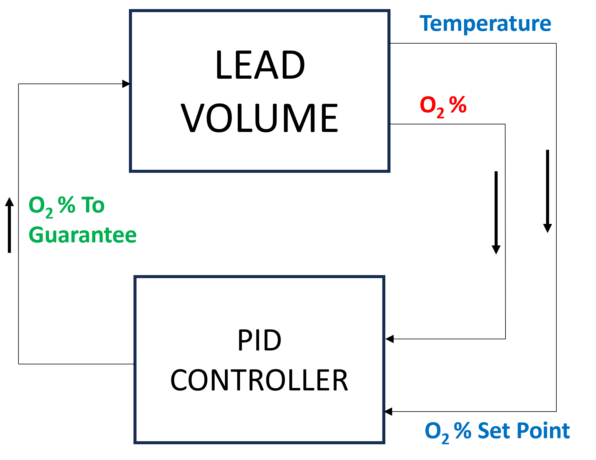
../_images/controlSchema.png — Fig. 2 Control schema of the oxygen concentration within the lead volume.

In detail:

the Lead Volume behaves as stated by the above mentioned heat balance equation, thus providing the actual temperature and oxygen concentration values;
the PID Controller estimates the oxygen concentration value to assure within the Lead Volume;
the setpoint the controller should follow is computed as the middle value of the admissibile oxygen concentration range, and it is computed by exploiting the actual temperature value of the Lead Volume;
the PID Controller tries to reach the setpoint value which changes in time according to the evolution of the Lead Volume.

This tutorial implements the just described system by extracting the thermo-physical and the thermo-chemical properties of the lead volume by means of the lbh15 package. The user can try more configurations than the one already implemented by changing the value of the following variables:

Lead initial temperature in \(\left[K\right]\);
Maximum value of the heat load applied to the lead volume in \(\left[W / m^3\right]\);
Time instant when the heat load changes instantaneously in \(\left[s\right]\);
Constant dissipated heat power in \(\left[W / m^3\right]\);
Oxygen initial concentration in \(\left[wt.\%\right]\);
PID controller settings, that is, the proportional, the integral and the derivative coefficients;
Simulation duration;
Number of integration time steps.

By looking into the code implementation, the following sections are identified:

Modules importing:
```
import numpy as np
from lbh15 import Lead # LBH15 package
from simple_pid import PID # PID controller
import support # Supporting functions
```
where:
- the lead-related module is imported from the lbh15 package;
- the PID module is imported from the simple_pid package, which is available at https://pypi.org/project/simple-pid/ and can be installed by applying the following instruction:
```
python -m pip install simple-pid
```
  simple-pid \(>= 2.0.0\) is required;
- the support module collects all the functions that are used in the remaining portion of the code; it imports the matplotlib package, which is available at https://pypi.org/project/matplotlib/ and can be installed by applying the following instruction:
```
python -m pip install matplotlib
```
  matplotlib \(>= 3.7.1\) is required;

Constant and initial values setting:

######
# Data
# Operating conditions
T_start = 800 # Initial lead temperature [K]
Qin_max: float = 2.1e6 # Maximum value of heat load [W/m3]
t_jump: float = 100 # Time instant when the heat load jump happens [s]
Qout: float = -1e6 # Value of dissipated heat power [W/m3]
Ox_start = 7e-4 # Initial oxygen concentration [wt.%]
# PID controller settings
P_coeff: float = 0.75 # Proportional coefficient [-]
I_coeff: float = 0.9 # Integral coefficient [-]
D_coeff: float = 0.0 # Derivative coefficient [-]
max_output: float = Ox_start # Maximum value of the output [wt.%]
# Simulation settings
start_time: float = 0 # Start time of the simulation [s]
end_time: float = 200 # End time of the simulation [s]
time_steps_num: float = 1000 # Number of integration time steps [-]

Declaration and initialization of support and solution arrays:
```
#####################
# Arrays of variables
# Time
time, delta_t = np.linspace(start_time, end_time, time_steps_num, retstep=True)
# Heat load time history
t_jump = t_jump if start_time < t_jump and end_time > t_jump else\
    (end_time-start_time)/2.0
Qin_signal = Qin_max * np.heaviside(time - t_jump, 0.5)
Qin = {t:q for t,q in zip(time, Qin_signal)}
# Lead temperature
T_sol = np.zeros(len(time))
# Oxygen concentrations
Ox_stp = np.zeros(len(time))
Ox_sol = np.zeros(len(time))
```
where:
- time contains all the time instants which the solution is computed at;
- delta_t is the integration time step;
- Qin is a dictionary containing for each time instant (key) the corresponding heat load value; values coincide with the Heaviside function values stored in Qin_signal;
- T_sol is the array where the lead temperature time history will be stored;
- Ox_stp is the array where the oxygen concentration setpoint values will be stored that will be followed by the PID controller;
- Ox_sol is the array where the oxygen concentration values will be stored that will be suggested by the PID controller;
Solutions initialization and lead object instantiation:
```
########################
# Set the initial values
T_sol[0] = T_start
lead = Lead(T=T_start)
Ox_stp[0] = support.ox_concentration_setpoint(lead)
Ox_sol[0] = Ox_start
```
where:
- lead object is instantiated at a reference temperature equal to the initial temperature of the lead volume;
- the initial value of the oxygen concentration setpoint is taken equal to the middle value of the admissibile operative range of the oxygen concentration as function of temperature;

PID controller setup:

########################
# Set the PID controller
pid = PID(P_coeff, I_coeff, D_coeff,
          setpoint=Ox_stp[0], starting_output=Ox_start/2)
pid.sample_time = None
pid.time_fn = support.sim_time
pid.output_limits = (0, max_output)

where:

the time function sim_time is imposed to the PID controller, that makes it operate in the simulation time framework;

Controller system evolution in time:

# Solve the balance equation in T and control the oxygen concentration
i = 1
for t in time[1:]:
    lead.T = T_sol[i-1]
    T_sol[i], Ox_stp[i], Ox_sol[i] = \
        support.integrate_in_time(lead, t, float(delta_t), Qin[t],
                                  Qout, Ox_sol[i-1])
    pid.setpoint = Ox_stp[i]
    Ox_sol[i] = pid(Ox_sol[i])
    i += 1

where there is a loop over all the required time instants; for each i-th instant:

an explicit call is made to the time integration function;
the oxygen concentration setpoint is updated correspondingly;
the PID is asked to provide the new oxygen concentration value to guarantee within the lead volume;

Results plotting:

#######
# Plots
# Qin signal
support.plotTimeHistory(1, time, np.array(list(Qin.values())),
                        "time [$s$]", "Qin [$W/m^3$]",
                        "Heat Load Time History",
                        "time_Qin.png")
# T_sol
support.plotTimeHistory(2, time, T_sol,
                        "time [$s$]", "T [$K$]",
                        "Lead Temperature Time History",
                        "time_T.png")
# Ox_sol overlapped to Ox_stp
support.plot2TimeHistories(3, time, Ox_sol, "Control",
                          time, Ox_stp, "Set-Point",
                          "time [$s$]", "Oxygen Concentration [$wt.\\%$]",
                          "Oxygen Concentration vs Setpoint Time History",
                          "time_OxVsOxStp.png")

where:

the first call to plotTimeHistory() returns the 2D plot shown in Fig. 1, where the heat load time history is depicted;
the second call to plotTimeHistory() returns the 2D plot where the temperature time history is depicted of the lead volume (see Fig. 3);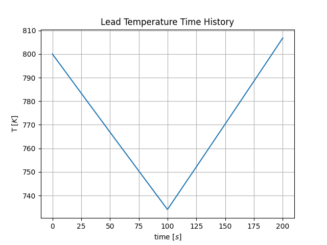

Fig. 3 Time evolution of the temperature of the lead volume.
the call to plot2TimeHistories() returns the 2D plot where both the oxygen concentrations time histories are reproduced, that is, the one of the setpoint and the one of the actual oxygen concentration (see Fig. 4);

Fig. 4 Time evolution of the oxygen concentrations within the lead volume: the oxygen concentration setpoint (orange) and the actual controlled oxygen concentration (blue).

After an initial transient, the blue curve, representing the controlled oxygen concentration within lead, overlaps almost exactly with the setpoint values (orange curve). The overlapping of the two oxygen concentration curves can be improved or worsened by varying the PID coefficients.

Note

This tutorial works even with the Bismuth and the LBE classes instances.

API Guide

This section contains a detailed description of the implementation of the main modules the lbh15 package is made of. lead Module, bismuth Module and lbe Module sections provide at first the list of the default correlations implemented in the corresponding lead-, bismuth- and lbe-related modules, and then the corresponding Application Programming Interface (API). In the end, in properties Modules section, the API Guide is provided of all the properties classes.

lbh15 Package