Getting started

This chapter presents all the information the user needs to make the best use of GLOW. Section Geometry Definition provides details about the available functionalities for setting up a geometry layout and displaying it in the 3D viewer of SALOME. Section Layout Export provides information about the process that GLOW automatically performs to generate the output .dat file containing the description of the geometry layout. In both sections, the available functionalities for building and exporting a geometry layout are described with code snippets showing their usage. Images are also provided to graphically present the results when displayed in the 3D viewer of SALOME. Lastly, section Usage gives indications about how to include the functionalities of GLOW in a Python script and how to run the script in the SALOME environment.

Geometry Definition

From a topological point of view, GLOW enables the construction of geometry layouts by exploiting several entities of the GEOM module of SALOME. The full list of GEOM entities is the following:

• vertex, which is a point in the XYZ space;

• edge, which can be classified as segment, arc of circle or circle;

• wire, a closed set of edges;

• face, a 2D area made from one or two wires;

• shell, made from a group of faces;

• solid, a 3D object made from a group of shells;

• compound, a container grouping together several GEOM entities.

GLOW relies on most of the above-mentioned topological entities to assemble the geometry layouts and visualise them in the 3D viewer of SALOME. The module geom_entities provides dedicated wrapper classes acting as an interface towards the topological entities of the GEOM module that are used in GLOW. All the layouts that can be built in GLOW inherit from one of these wrapper classes, which all derive from the GeomWrapper base class. This class has been implemented so that attribute access is delegated to the underlying wrapped GEOM object (identified as GEOM_Object). This design choice allow for its subclasses to behave like the GEOM_Object they refer to. As a result, these classes can be used with any GEOM function directly without the need for the user to provide the corresponding GEOM_Object. In addition, the GeomWrapper class overloads the following arithmetic operators to easily perform Boolean operations between instances of this class:

• + (__add__) performs a fuse (union) of two shapes.

• - (__sub__) performs a cut (difference) of one shape with another one.

• * (__mul__) produces the common (intersection) part of two shapes.

• / (__truediv__) perform a partition operation where the first GEOM_Object is subdivided in sub shapes by given shape objects.

• // (__floordiv__) perform a partition operation where the resulting shape is the combination of all the shapes after being partitioned.

These operators call the corresponding wrapper functions of the GEOM ones provided in the geom_interface module that perform the Boolean operations. In addition to these functions, the module also contains functions for building the GEOM topological entities and applying operations to them (e.g., Euclidean transformations).

In GLOW, the base class from which all the classes identifying any layout derive from is the Layout class. It provides the characteristic data and behaviour (in terms of methods) every layout object should have. In particular, instance methods for applying Euclidean transformations, displaying and updating the corresponding GEOM_Object are declared but left empty. Subclasses of Layout, which represent geometric objects describing the layout of cells and lattices, provide dedicated implementations for these methods. The available common methods are:

• rotate(). It rotates the layout by a given angle (in degrees) around the given axis, if any is provided, otherwise around the central perpendicular axis.

• scale(). It scales the layout by a given factor from a given vertex or the layout’s centre, if not provided.

• show(). It displays the GEOM_Object the instance refers to in the 3D viewer of SALOME according to specific settings.

• translate(). It translates the layout in the XYZ space so that its centre coincides with the point identified by the given coordinates.

• update(). It allows to update the GEOM_Object the instance refers to with a new one. The object to update with is given in terms of objects of the Face and Compound classes.

The following classes are direct children of Layout:

• Surface. It represents the base class for all the geometric shapes used in GLOW to describe the surfaces a geometry layout is made of. In geometric terms, it describes a 2D surface, and, for this reason, it also derives from the Face wrapper class. Dedicated classes to easily build specific geometric shapes (i.e. circles, rectangles and hexagons) are children of this class.

• Region. It represents any 2D surface that is filled by a set of properties, like the material. This class inherits also from the Face wrapper class.

• Fillable. It represents any geometry layout that can be filled with several regions, each associated to a set of properties. It is an abstract class that inherits from the Compound wrapper class since it groups several GEOM faces together.

The building concept adopted in GLOW to describe any geometry layout of cells and lattices is based on the layers idea. Layers are meant to represent the layout as a hierarchical tree where the leaves are constituted by Region instances, while the nodes are given by instances of the Fillable subclasses. Each subclass of Fillable (i.e. cells and lattices) implements the layers concept. This means that, as an example, a cell can represent a node in the hierarchical tree of a lattice, but the same can be said for a lattice, when included in the tree of a cell that describes an assembly. The Fillable subclasses provide methods for inserting regions or other fillable objects into the layout’s ordered layer structure. The insertion order determines each object’s position in the hierarchical tree, where the layer index defines its rendering priority within the layout. Consequently, objects added earlier are placed in lower layers, while objects added later occupy progressively higher layers. The most recently inserted elements therefore appear at the top of the layout’s Z-ordering. In this sense, the layer abstraction provides a mean for imposing an ordering of geometric objects along a conceptual Z-axis (even if the resulting layout is always 2D), ensuring proper handling of overlapping shapes based solely on insertion order.

When geometry layouts are displayed or exported, their hierarchical tree is traversed from the highest filled layer down to the lowest (i.e. from top to bottom). During this traversal, any region or fillable located in a lower layer that is overlapped by an element in a higher layer is either clipped (if partially overlapped) or removed entirely (if fully covered).

The placement of region or fillable objects within a geometry layout relies on Euclidean geometric transformations, such as translation and rotation. Assembling the entire layout resulting from collapsing the layers is based on Boolean operations (i.e. intersection, cut and partitioning).

In GLOW, the geometry layout of Fillable objects (i.e. cells and lattices) is described in terms of:

• the technological geometry, in which regions delineate areas each associated with a specific material;

• the sectorised geometry, which further subdivides the regions of the technological geometry into sectors and circular areas. This refined geometry is typically used to capture flux gradients arising from geometric heterogeneities. An instance attribute in the fillable classes stores the association between the GEOM compound of edges resulting from the refinement with the type of geometry (i.e. the GeometryType.SECTORIZED).

Fillable objects can be displayed in the 3D viewer of SALOME in terms of one of the aforementioned types of geometry. This is performed automatically by traversing the hierarchical tree to collect all the corresponding geometry layouts.

GLOW allows users to display the regions of a geometry layout according to a colour map associated to a specific property type. Given the hierarchical structure of a fillable, its layers are traversal to collect all the Region objects coming for the current fillable and from those representing the nodes of the layout’s tree. Each Region instance associates its GEOM face (part of the technological geometry layout) with a colour that corresponds to the value of the property type to be visualised in the 3D viewer of SALOME.

Users can assign values (as a string) for the type of properties available from the PropertyType enumeration to any Region object. These property types include:

• MATERIAL, to indicate the name of the material.

• MACRO, to indicate the name of the macro. Regions can be grouped together in a macro region to enable support for the multicell surfacic approximation in DRAGON5.

Information about the MATERIAL property, in terms of its assigned values and indices for the regions, is always included in the output file when the geometry is exported. The names and indices of the macro regions are included only if indicated by the user (see Layout Export).

The specific classes associated to cells and lattices, which can be used to model assemblies, and even the entire core, are the following ones:

• Cell. It represents a generic cell that is not based on a pre-defined characteristic shape, which is provided at its initialisation.

• CartesianCell. It represents a Cartesian cell, i.e. one having a rectangular surface as its characteristic shape.

• HexCell. It represents a hexagonal cell, i.e. one having a hexagonal surface as its characteristic shape.

• Lattice. It represents a generic lattice that do not follow a specific pattern.

• CartesianLattice. It represents a Cartesian lattice made of cells arranged according to a rectangular grid.

• HexLattice. It represents a hexagonal lattice where cells are arranged on a hexagonal grid.

All the aforementioned classes inherit from the Fillable class, which means that they all share the same common methods devoted to the management of the hierarchical tree, the addition of layout objects, the application of Euclidean transformations and symmetry operations, and to displaying the geometry layout in the 3D viewer of SALOME. In addition, they are based on a characteristic shape (i.e. an object of the Surface subclasses) which, depending on the layout type, is a rectangular or a hexagonal surface, or a generic surface derived from the borders of the layout.

In the following, the different layout objects are discussed and their public methods are detailed.

Surfaces Definition

GLOW comes with classes to quickly build specific surfaces, identified by GEOM faces, in SALOME. In the Object-Oriented Programming (OOP) view, the types of surface that are available in GLOW inherit from the same superclass Surface, which represents a generic 2D shape in SALOME. Subclasses of Surface are present in GLOW to build specific-type surfaces. They are the following:

• class Circle for circular surfaces.

• class Hexagon for hexagonal surfaces.

• class Rectangle for rectangular surfaces.

Depending on the specific type of surface, the instantiation requires to specify the centre of the surface and its characteristic dimensions (i.e. radius for a circle, width and height for a rectangle, the edge length for a hexagon) or the 2D shape and the centre directly (Surface case). Classes are implemented with default values for the characteristic dimensions. When an object of the Surface subclasses is instantiated, the GEOM objects that concur in the creation of the corresponding face are automatically built. In this way, the surface can be shown in the SALOME 3D viewer right after the initialization by means of the method show().

The following code snippet shows how to instantiate and display the geometric surface for the hexagonal case.

from glow.geometry_layouts.geometries import Hexagon

surface = Hexagon(center=(1.0, 1.0, 0.0), edge_length=2.0)
surface.show()

Fig. 1 shows the graphical result obtained by running the above code in a Python script or directly from the Python console of SALOME.

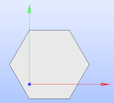
Fig. 1 Hexagon displayed in the SALOME 3D viewer.

As mentioned in Geometry Definition, Euclidean transformations are common to all classes of GLOW that inherit from Layout. The Surface class provides a specific implementation for these methods that is shared by all its subclasses. In particular, the rotate(), translate() and scale() methods apply a rotation, translation and scaling, respectively, to the GEOM elements of the Surface instance.

For the hexagonal surface declared above, the code instructions are the following:

surface.rotate(90)
surface.translate((0.0, 0.0, 0.0))
surface.scale(0.5)
surface.show()

By applying these methods, the resulting GEOM face is shown in Fig. 2, and compared with the original shape.

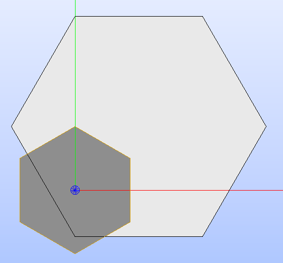
Fig. 2 Hexagon before and after applying rotation, traslation and scaling operations.

The GEOM face that is specific of the subclass of Surface can be directly modified within SALOME and the modified GEOM face applied to the Surface subclass object by calling the method update(). The implementation of this method is specific for each of the subclasses of Surface. In general, the method receives as parameter a GEOM face and updates the instance attributes of Surface accordingly. A check ensures that only GEOM faces are provided, and that the given GEOM face corresponds to the characteristic surface the Surface class refers to.

Region Definition

In GLOW, the geometry layouts are described as a hierarchical tree in which the regions are the leaves. The class that implements the region concept is Region. This class represents any 2D shape bounded by one or two edges that is filled by a set of properties, e.g. the material. Properties are expressed as a dictionary of items of the PropertyType enumeration vs the corresponding names. As any other geometric object in GLOW, the Region class inherits from a subclass of the GeomWrapper, specifically the Face one. This guarantees that Region instances behave like the corresponding GEOM face objects when used with GEOM functions. As mentioned in Geometry Definition, the Region is a subclass of Layout, meaning it provides the implementation for all the methods handling Euclidean transformations, displaying and updating the region. In addition, to enable the visualisation of the regions of a layout according to a property type colour map, Region objects come with a dedicated color attribute and methods for setting (set_region_color()) and resetting (reset_region_color()) the colour according to which it is displayed in the 3D viewer of SALOME. When the region’s colour is reset, it is assigned the default RGB colour used by SALOME, which corresponds to a light grey. The Region class comes also with the clone() method for producing a copy of the instance that is completely independent from the source instance, but has the same properties and colour.

The Boolean algebra provided by overloading the arithmetic operators of Python in the GeomWrapper class is complemented in the Region class by providing specific implementations for the following operators:

• + (__add__) fuses the GEOM faces of one or more regions while keeping the same properties. Both regions must have the same values for the properties.

• * (__mul__) produces the common (intersection) part of the GEOM faces of two regions while keeping the same properties of the region that intersects the first one.

The instantiation of a Region object is based on a GEOM face, but it also accepts an instance of the Surface class as it accesses to the wrapped GEOM face. The following snippet shows the creation of two regions with dedicated properties, the assignment of a colour and their visualisation in the 3D viewer. The association of colours to regions according to the values of a given PropertyType is performed by means of the associate_colors_to_regions(). Fig. 3 shows the result of applying the Boolean operations, identified by the arithmetic operators, to the two regions.

from glow import *

# Instantiation of the two regions
r1 = Region(
  Hexagon(), "R1", {PropertyType.MATERIAL: "MAT1"}
)
r2 = Region(
  Hexagon(center=(1,1,0), edge_length=2.0),
  "R2",
  {PropertyType.MATERIAL: "MAT2"}
)

# Get the common part
r3 = r2 * r1
r3.name = "R3"
# Clone the first region and set its material to be
# the one of the second region
r4 = r1.clone()
r4.name = "R4"
r4.properties[PropertyType.MATERIAL] = "MAT2"
# Fuse the second and fourth regions
r5 = r2 + r4
r5.name = "R5"
# Associate colours to the regions according to the material
regions = [r1, r2, r3, r4, r5]
associate_colors_to_regions(PropertyType.MATERIAL, regions)
for region in regions:
  set_color_face(region.geom_obj, region.color)

# Display all the regions
r1.show()
r2.show()
r3.show()
r4.show()
r5.show()

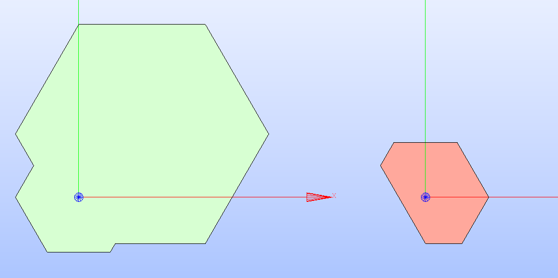
Fig. 3 Region resulting from fusing (on the left) and intersecting (on the right) two regions.

Fillable Definition

According to the hierarchical tree logic adopted in GLOW, classes that inherit from the Fillable class are the nodes in the tree, as they represent a container for other nodes or leaves. The superimposition of multiple layers filled with either Region or other Fillable objects recreates the hierarchical structure.

Fillable inherits from the Compound wrapper class, as it represents a collection of GEOM faces. In addition, it can be used as argument of the GEOM functions directly, as it behaves like the corresponding GEOM compound object when used with GEOM functions. As mentioned in Geometry Definition, Fillable is a subclass of Layout, meaning it provides the implementation for all the methods handling Euclidean transformations, displaying and updating the layout it refers to.

The class Fillable declares attributes and methods common to all its subclasses. Public methods cover the following functionalities:

• adding a new region or fillable to the geometry layout;

• applying a specific symmetry type to the geometry layout;

• cloning the instance;

• getting the compound of edges that corresponds to a given item of the GeometryType enumeration;

• getting the Region objects the geometry layout (either full or the one corresponding to a specific symmetry) is made of;

• printing information about a region, either given or selected from the SALOME GUI;

• restoring the geometry layout;

• rotating, scaling and translating the instance;

• setting the properties of a region, either given or selected from the SALOME GUI;

• displaying the geometry layout in the 3D viewer;

• updating the GEOM_Object the instance refers to;

• updating the hierarchical structure of the instance.

Adding a new layout

The method add() allows for the inclusion of a new Region or Fillable object to the hierarchical tree that describes the technological geometry layout of the current fillable. Users can provide also the XYZ coordinates at which the object should be placed at, as well as the index of the layer in which the object is added. A translation is performed, if needed, to place the layout object so that its CoG coincides with the given coordinates. If no position is provided, the layout object is placed in the CoG of the current fillable.

The given layout object is stored at the last position of the layer identified by the given index, if any is provided. This means that the object is added as the last element in the corresponding sublist of the glow.geometry_layouts.fillable_layouts.Fillable.layers attribute. If no index is provided, the layout object is added to a new sublist of layers.

This method simply updates the list of layers of the technological geometry layout of the current fillable with the given layout object without collapsing the layers and updating the entire GEOM compound object. To update the hierarchical tree of the fillable by cutting overlapping layers, the method update_hierarchical_structure() should be called. To update and display the fillable in the 3D viewer of SALOME, the method show() should be run instead.

The following snippet shows the usage of the method add() when applied to a CartesianCell to include:

• a circular Region object, being a region of material;

• a CartesianLattice object, to model an assembly of cells. For the construction of a Cartesian lattice, see Lattice Definition.

Results are shown in Fig. 4 for both a single cell and an assembly.

from glow import *

# Instantiation of a circular region, a cell and a lattice of cells
r1 = Region(
  Circle(radius=0.3), "R1", {PropertyType.MATERIAL: "MAT1"}
)
cell = CartesianCell(base_props={PropertyType.MATERIAL: "MAT2"})
cell.add(r1)
lattice = CartesianLattice()
lattice.add_rings_of_cells(cell, 3)

# Instantiate the cell representing the assembly
assembly = CartesianCell(
  width_height=tuple(i+1 for i in lattice.dimensions),
  base_props={PropertyType.MATERIAL: "MAT2"}
)
# Add the lattice to the assembly cell
assembly.add(lattice)

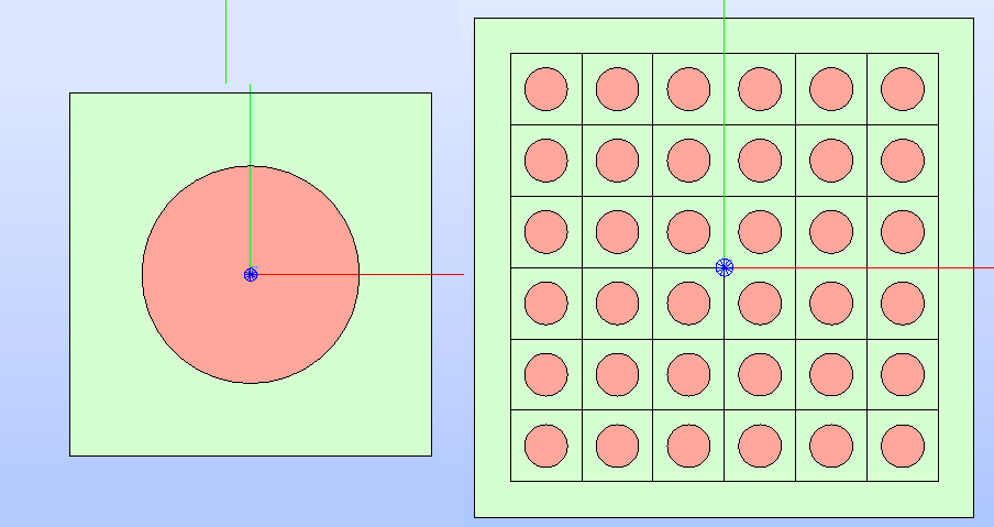
Fig. 4 Technological geometry layout after adding a single Region (on the left) and a fillable CartesianLattice (on the right).

Applying a symmetry

Solving the Boltzmann transport equation on a full geometry layout can be computationally expensive, in particular if very complex. To speed up the calculations, users can rely on cuts to extract parts out of the existing layout, thereby isolating the minimum portion of the geometry required to describe the entire pattern. GLOW supports the application of specific types of symmetries to any fillable object that inherits from Fillable.

The method apply_symmetry() allows users to apply a symmetry type by indicating an item of the enumeration SymmetryType. According to the type, the 2D shape that identifies the symmetry is derived and stored in the symmetry_map instance attribute; this is a dictionary associating to each SymmetryType element the corresponding Surface instance. The indicated symmetry type is saved in the state attribute and applied when the current fillable is displayed in the 3D viewer or exported to file in the TDT-compatible format. In both cases, a common operation is performed between the Region objects identifying the entire geometry layout and the shape of the symmetry. Only the regions and parts of them that are in common are kept and either displayed or exported.

The method apply_symmetry() only supports a set of SymmetryType elements that are common to all fillable objects. These types are the following ones:

• FULL: the characteristic shape of the entire layout is stored.

• HALF: a rectangular shape representing half of the entire layout is stored.

• QUARTER: a rectangular shape representing one quarter of the entire layout.

Subclasses of Fillable provide the implementation to handle type-specific symmetries (see Applying cell’s type-specific symmetries).

The following code snippet shows the application of a QUARTER symmetry type for a Cartesian assembly. The result is shown in Fig. 5.

assembly.apply_symmetry(SymmetryType.QUARTER)

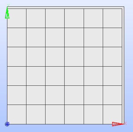
Fig. 5 Cartesian lattice after applying the QUARTER type of symmetry.

Users should note that even if called from the SALOME Python console, the method apply_symmetry() does not automatically update and display the portion of the geometry layout that corresponds to the applied symmetry. To display the new layout, the method show() must always be called. In addition, the last applied symmetry is not used when the current Fillable object is exported. It is up to the user to indicate the symmetry type to the function exporting the layout (see Layout Export).

Cloning the fillable instance

The Fillable class comes with the clone() method for producing a copy of the current instance that is completely independent from the source instance. In Python terms, this means making a deep copy. This allows the mutable attributes (e.g., lists and dictionaries) of a cloned fillable to be unlinked from the source fillable. This means that modifications to a mutable attribute in one fillable are not also performed in the corresponding attribute of the other fillable.

Getting the geometry type edges

As mentioned in Geometry Definition, Fillable objects are described in terms of the technological geometry, collecting the regions each associated to a material, and the sectorised geometry, which represents the refinement of the former geometry layout.

The Fillable class stores the refined geometry layout as a Compound object collecting the edges that subdivide the regions resulting by applying a sectorisation (see Sectorization Operation).

Since a Fillable object possesses a hierarchical structure, when displaying the root fillable in terms of the sectorised geometry (see Displaying the geometry layout), the Compound objects identifying the sectorised geometry of all the fillables in the hierarchy tree of the current istance are retrieved. The method get_geometry_map() iterates over all the tree to collect all the sectorised geometries in a single Compound object of edges. This method is useful for updating the geometry_maps, a dictionary associating for each element of the GeometryType the corresponding Compound object of edges. Currently, it can stores only the edges of the sectorised geometry.

The following snippet shows how to update the compound of edges corresponding to the SECTORIZED type of geometry when a sectorisation has already been applied to a Cell instance.

# Collect the refined geometry of the cells and join it with the mesh
# by performing a partition
assembly.geometry_maps[GeometryType.SECTORIZED] = \
    assembly.get_geometry_map(GeometryType.SECTORIZED) // wrap_shape(mesh)

# Show the resulting refined layout with the 'MATERIAL' colour map
assembly.show(PropertyType.MATERIAL, GeometryType.SECTORIZED)

For a deeper insight, please refer to the Cartesian Assembly With Symmetry use case in the Tutorials section (see Fig. 23 for the resulting refined geometry).

Getting the regions

In GLOW, objects of the Region class represent the leaves of the hierarchical tree of a fillable object. When an instance of the Fillable subclasses is either displayed or exported, GLOW automatically retrieves the regions of the technological geometry. The methods get_regions() and get_regions_with_symmetry() serve to this purpose. The former method iterates over all the layers of the current fillable to collect and return all the Region objects that describe the technological geometry layout. The regions are collected directly from the current fillable and by recursively calling the get_regions() method for all the Fillable objects in the hierarchy.

The method get_regions_with_symmetry() similarly retrieves the regions of the technological geometry, with the difference that only those in common with the shape of the indicated symmetry type are returned. The underlying common operation can introduce numerical floating-point precision errors. To limit the effect, this method includes a boolean flag to specify whether the tolerances of the geometric elements of the Regions objects should be limited to the 1e-6 value.

Printing regions information

When the geometry layout of a fillable is displayed in the 3D viewer of SALOME, GLOW retrieves and adds to the SALOME study the GEOM face of all the Region objects that identify the technological geometry.

Users can obtain information about the Region object that corresponds to either the given GEOM face or the one currently selected in the 3D viewer. The method print_region_info(), when called directly in the Python console of SALOME, prints the following data (see Fig. 6):

• the tree representation of the hierarchical structure up to the target Region object;

• the code to retrieve the target Region object directly from the hierarchical tree of the current fillable;

• the values for each of the PropertyType items associated to the target Region object.

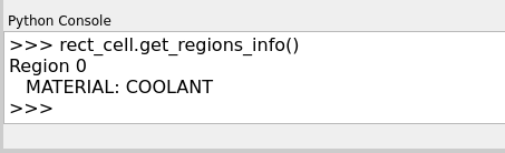
Fig. 6 Information about the Region object that corresponds to the GEOM face of the fillable currently selected in the 3D viewer of SALOME.

Restoring the geometry layout

There could be cases in which users need to reset the technological geometry of a fillable by removing all the regions and clearing all the properties (see Hexagonal Assembly With Different Cells). The restore() method addresses this need by clearing the layers attribute from any Region and Fillable object previously stored. In addition, any symmetry and geometry types mappings (i.e. the symmetry_map and the geometry_maps attributes) are completely cleared.

A GEOM face object is built from the shape of the technological geometry of the fillable to restore; the layers and the regions attributes are filled only with the Region object built from this GEOM face. However,no properties are associated to this new region.

Applying Euclidean transformations

As mentioned in Geometry Definition, Euclidean transformations are common to all classes of GLOW that inherit from Layout. The Fillable class provides a specific implementation for these methods that is shared by all its subclasses.

In particular, the rotate(), translate() and scale() methods apply a rotation, translation and scaling, respectively, to the following elements:

• the py:class:Region<glow.geometry_layouts.layouts.Region> and py:class:Fillable<glow.geometry_layouts.fillable_layouts.Fillable> objects stored in the layers attribute;

• the GEOM_Object the current fillable refers to;

• the Compound objects of the geometry_maps attribute;

• the Face objects of the symmetry_map attribute.

Users should note that even if called from the SALOME Python console, the methods applying the Euclidean transformations does not automatically display the updated geometry layout. To do so, the method show() must always be called.

Setting properties

Values for the elements of the PropertyType enumeration are associated to the Region objects that constitute a fillable. In GLOW, properties are assigned directly when instantianting a Region object, a Cell one or any of its subclasses. In case of a Cell, properties are assigned to the Region object built from the characteristic shape of the cell.

To set or update the value for a specific property type of a Region object belonging to the hierarchical tree of the current fillable, the method set_region_properties() is available for all subclasses of Fillable. This method allows users to set values for the indicated property types for the Region object of the fillable whose GEOM face is provided as input. If none is given, the GEOM face currently selected in the 3D viewer is considered. The whole hierarchical tree of the fillable is traversed to find the Region object that matches the GEOM face. If found, the corresponding properties attribute is updated.

The following code snippet shows how to set values for the MATERIAL type of property to a circular region whose properties was not defined at its instantiation. For the construction of a Cartesian cell, see Cell Definition.

# Build the cell's geometry layout by adding two circular regions
cell = CartesianCell(
    name="Cartesian cell", base_props={PropertyType.MATERIAL: "MAT_1"}
)
for radius, mat in zip([0.4, 0.3], ["MAT_2", "MAT_3"]):
    cell.add(
        Region(
          Circle(radius=radius), properties={PropertyType.MATERIAL: mat}
        )
    )
# Add a new circular region without any property
circle = Circle(radius=0.2)
cell.add(Region(circle))
# Set the circular region properties
cell.set_region_properties(
    {PropertyType.MATERIAL: "MAT_4"}, circle
)
# Display the cell
cell.show(PropertyType.MATERIAL)

In particular, materials are assigned to the characteristic shape of the Cartesian cell and to the regions directly. A new circular region is then added, and the corresponding Circle instance is used to identify the region of the cell whose material property needed to be assigned. From within the SALOME 3D viewer, the region can be provided by simply selecting the corresponding GEOM face and calling the method from the integrated Python console. In any case, the cell’s geometry layout with the MATERIAL colour map is shown in Fig. 7.

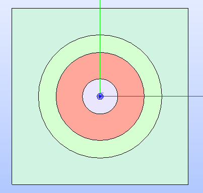
Fig. 7 Cartesian cell after setting up values for the MATERIAL property type for each region. It is shown with a colour map highlighting the different values assigned to the cell’s regions.

The following example shows how to set the MACRO property to the regions of a hexagonal assembly, modelled as a HexCell containing a HexLattice. For details about the construction of a lattice of cells, please refer to Lattice Definition.

from glow import *

# Build the lattice geometry layout
hex_cell = HexCell()
hex_cell.add(Region(Circle(radius=0.3)))
hex_cell.rotate(90)
lattice = HexLattice([hex_cell])
lattice.add_ring_of_cells(hex_cell, 1)
# Build the assembly so that it is slightly greater than the lattice
assembly = HexCell(side=1.1*lattice.dimensions[0])
assembly.add(Region(Hexagon(edge_length=lattice.dimensions[0])))
assembly.add(lattice)
assembly.update_hierarchical_structure()
# Assign the 'MACRO' property so that the box layer and the background has
# the same value, whereas each cell of the lattice has a different value
assembly.set_region_properties(
    {PropertyType.MACRO: "MAC_001"},
    assembly.layers[0][0]
)
# Loop through the regions of the background of the assembly
for region in assembly.layers[1]:
    assembly.set_region_properties(
        {PropertyType.MACRO: "MAC_001"}, region
    )

macro_index = 1
# Loop through the layers of the lattice, and through those of each cell
for layer in assembly.layers[2][0].layers:
    for cell in layer:
        # Increment the macro index for each cell
        macro_index += 1
        for cell_layer in cell.layers:
            for cell_region in cell_layer:
                cell_region.properties = \
                    {PropertyType.MACRO: "MAC_00" + str(macro_index)}

# Show the assembly regions according to the 'MACRO' colour map
assembly.show(PropertyType.MACRO)

The resulting geometry layout of the assembly with the MACRO colour map is shown in Fig. 8.

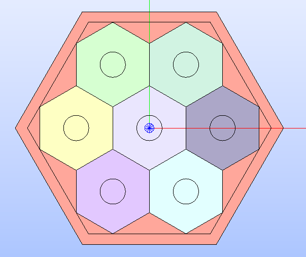
Fig. 8 Assembly after setting up the values for the MACRO type of property. It is shown with the corresponding colour map.

Displaying the geometry layout

The geometry layout of any of the Fillable subclasses can be displayed in the 3D viewer of SALOME by calling the method show(). This method erases all the previously shown GEOM objects from the view, and removes the GEOM compound that corresponds to the technological geometry layout of the current fillable. Its hierarchical tree is then updated, if needed, to cut any overlapping layer still not handled. The GEOM_Object (i.e. a GEOM compound) that corresponds to the technological geometry layout of the current fillable is added to the SALOME study and displayed in the 3D viewer.

In addition, the method retrieves the Region objects (which are representative of the technological geometry layout), and, if necessary, applies the common operation with the currently active type of symmetry. The GEOM face of each region is added to the SALOME study and included in the Object Browser as children of the GEOM_Object of the fillable. If not displayed automatically, these GEOM faces can be shown all at once by selecting the “Show Only Children” item in the contextual menu (see Fig. 9).

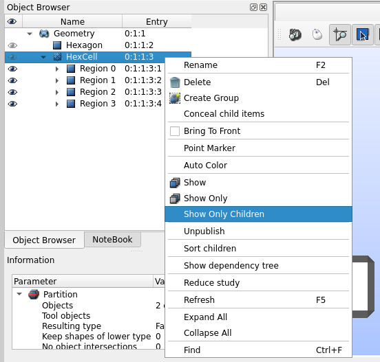
Fig. 9 How to display the regions associated to a cell in SALOME.

The show() method displays the regions according to a colour map based on the values assigned to each region for the provided element of the enumeration PropertyType. The RGB colours of the map are randomly generated and uniquely associated to the values of the indicated element of PropertyType that each region stores in the properties attribute. If no property type is provided, the regions are displayed with a default colour.

By default, the show() method displays the regions of the technological geometry. If a different item of the GeometryType enumeration is given (i.e. the SECTORIZED one), the method also shows the Compound of edges of the refined geometry. This Compound object is retrieved from the refined geometry layouts of all the fillable objects in the hierarchical tree of the current one, extracting the common part with the shape of the symmetry currently applied, if needed. The resulting GEOM compound is added to the SALOM study, and, in the Object Browser, appears as a child of the GEOM_Object of the fillable.

The following code snippet shows how to display the refined geometry layout of a HexCell instance by applying a colour map according to the MATERIAL property type. Fig. 10 presents the resulting geometry layout as displayed in the 3D viewer of SALOME.

hex_cell.show(PropertyType.MATERIAL, GeometryType.SECTORIZED)

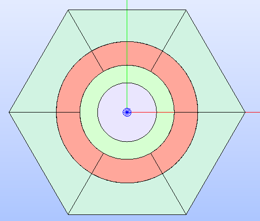
Fig. 10 Refined geometry layout of a hexagonal cell. Regions are displayed according to the MATERIAL colour map.

By default, the show() method automatically displays the GEOM faces of all the Region objects of the fillable. If specified differently by providing a boolean flag with value False, this method only adds the GEOM faces for the regions and the GEOM compound of edges of the refined geometry layout to the SALOME study without triggering their visualisation in the 3D viewer. This setting can be used to avoid overheads when geometry layouts characterised by many GEOM face objects are shown in SALOME.

Updating the GEOM_Object

The method update() allows users to update the GEOM_Object of the Fillable instance with another GEOM_Object provided in terms of a Compound or a Face object. This method also updates the centre of the layout (i.e. the o attribute) and any Compound object of edges associated to a GeometryType item.

Users should note that this method does not update the regions and fillables stored in the layers attribute accordingly with the updated GEOM_Object.

Updating the hierarchical tree

As described in Geometry Definition, the building concept of GLOW is based on the layers logic to model the hierarchical tree of a fillable. Whenever objects of the Fillable subclasses are displayed in the 3D viewer of SALOME or exported to file in the TDT-compatible format, the method update_hierarchical_structure() is automatically called.

This method traverses the entire hierarchical tree in reverse order to handle any region and fillable of a layer that is overlapped by a layer in a higher position along the conceptual Z-axis brought by the layers attribute. During this traversal, any region or fillable that is overlapped by a higher layer is either clipped (if partially overlapped) or removed entirely from the hierarchical tree (if fully covered). This operation is skipped and the method exits without changes if there is no need to update the layers of the fillable.

The operation of assembling all the layers requires that each node in the hierarchical tree is up-to-date. This means that each Fillable object found in the layers attribute is further processed by recursively calling this method to update its hierarchical structure.

Lastly, the GEOM_Object representative of the current fillable is updated by collecting in a GEOM compound all the Region objects retrieved from each layer.

To simplify the hierarchical tree, a True value can be provided to the update_hierarchical_structure() method. If so, the hierarchical tree of the fillable is collapsed and its layers reduced to a sigle layer collecting all the Region objects of the fillable. Users should note that any previously stored Fillable object is completely removed from the hierarchical tree and substituted with its Region objects.

Cell Definition

GLOW comes with classes to build cells having a generic, a hexagonal or a rectangular characteristic surface. According to the hierarchical tree logic, cells are the nodes as they inherit from the Fillable abstract class. The module glow.geometry_layouts.cells provides the base class Cell, which represents a cell characterised by a generic 2D shape, described from a Surface instance, or any of its subclasses.

The subclasses of Cell are the following ones:

• class CartesianCell for representing rectangular cells.

• class HexCell for representing hexagonal cells.

When instantiating any of the aforementioned subclasses, the corresponding instance of the Surface subclasses is built from the characteristic dimensions. For the generic Cell class, the initialisation is done from any 2D shape. The following code snippet shows how to instantiate the different type of cells available in GLOW.

from glow.geometry_layouts.cells import CartesianCell, Cell, HexCell

rect_cell = CartesianCell(
    center=(0.0, 0.0, 0.0),
    width_height=(1.0, 2.0),
    rounded_corners=[(1, 0.1), (3, 0.1)],
    base_props={PropertyType.MATERIAL: "MAT"},
    name='RectCell'
)

hex_cell = HexCell(
    center=(0.0, 0.0, 0.0),
    side=2.0,
    base_props={PropertyType.MATERIAL: "MAT"},
    name='HexCell'
)

gnrc_cell = Cell(
  shape=surface,
  base_props={PropertyType.MATERIAL: "MAT"}
)

For a Cartesian cell, the rounded_corners parameter indicates the index of the corner of the rectangle and the associated curvature radius to generate a rectangle with rounded corners. The base_props parameter allows to indicate the name of the properties that are associated to the characteristic shape of the cell. After the initialisation, the hierarchical tree of the cell contains a single Region object made from the GEOM face of the characteristic shape and the specified properties.

The classes for representing a cell in a geometry layout, besides inheriting attributes and methods from the Fillable superclass, declare a public method for handling the sectorisation operation. In addition, each provides its own implementation for deriving the shape of the symmetry according to the cell-specific symmetry types.

Sectorization Operation

As mentioned in Geometry Definition, the geometry layout of a Fillable, and, consequently, any Cell and its subclasses instances, can be refined by subdividing the regions of the technological geometry into a specified number of sectors. Cell and its subclasses share the same internal implementation for handling the sectorisation operation by deriving the GEOM compound of edges identifying the sectors (see sectorize()). In addition, the sectorize() method for the CartesianCell class has the option of applying the windmill sectorization to the region farthest from the cell’s centre, provided that the region is subdivided into eight or sixteen sectors.

The sectorisation operation is configured by providing two lists to the sectorize() method, one containing the number of sectors into which each cell-centred region has to be split, the other the angle (in degrees) the subdivision should start from wrt the X-axis. The order of the elements in the two lists follows the outwards direction from the cell’s centre. The sectorize() method for a Cartesian cell also accepts the windmill parameter, a Boolean flag indicating whether the wings of the windmill sectorization are derived.

The GEOM edges describing the sectorization are built so that they propagate radially from the centre of the cell. The result of the intersection between each region and the subdivision edges is collected in a Compound object and stored as entry in the geometry_maps dictionary for the SECTORIZED type of geometry.

The following code snippet shows how to apply a sectorization, with windmill option enabled, for a Cartesian cell having two cell-centred circles. Fig. 11 shows the result after applying the indicated sectorization.

rect_cell.sectorize([1, 4, 8], [0, 45, 22.5], windmill=True)
rect_cell.show(GeometryType.SECTORIZED)

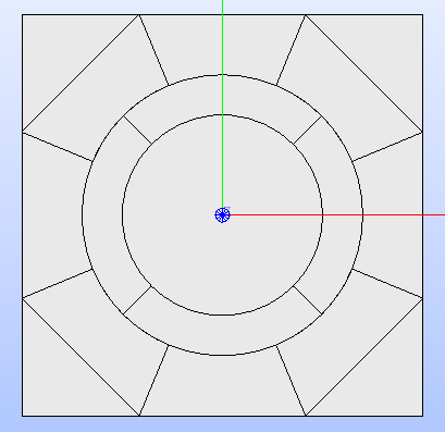
Fig. 11 Cartesian cell after applying the sectorization operation.

Applying cell’s type-specific symmetries

As mentioned in the Applying a symmetry section, the method apply_symmetry by default supports the construction of the shape of the symmetry associated to the FULL, HALF and QUARTER types.

In addition to the aforementioned common symmetry types, the CartesianCell class supports the following ones:

• EIGHTH: a right triangular shape representing one eighth of the entire cell;

• DIAG: a right triangular shape representing a half of the entire cell cut along the diagonal of its characteristic shape.

The HexCell class, besides the common symmetry types, supports also the following ones:

• THIRD: a parallelogram representing one third of the entire cell;

• SIXTH: a regular triangular shape representing one sixth of the entire cell;

• TWELFTH: a right triangular shape representing one twelfth of the entire cell.

Independently from the cell type, the result is the construction of a 2D shape used to derive the Region objects in common with the shape of the symmetry. For more details, please refer to the Applying a symmetry section.

Fig. 5 and Fig. 12 show the results of applying a QUARTER and a TWELFTH symmetry to a Cartesian and a hexagonal assembly, respectively.

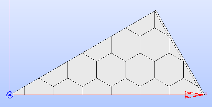
Fig. 12 Hexagonal assembly after applying the TWELFTH type of symmetry.

Lattice Definition

GLOW comes with classes to build lattices according to a generic, a Cartesian and a hexagonal pattern of the cells. According to the hierarchical tree logic, cells are the nodes as they inherit from the Fillable abstract class. The module glow.geometry_layouts.lattices provides the base class Lattice to represent any lattice made of cells without the need to follow a specific pattern. For this reason, this class can be used to model a portion of a generic lattice assembled by positioning the cells at the indicated coordinates.

Subclasses of Lattice present type-specific patterns:

• class CartesianLattice for representing a Cartesian pattern of cells.

• class HexLattice for representing a hexagonal pattern of cells.

The Lattice class and its subclasses can be instantiated either with or without providing a list of Cell objects. The method add() inherited from the Fillable superclass can be used to include the cells. Dedicated methods for adding one or more rings of cells at once are present as well (see Adding cell(s)).

The following code snippet shows how to instantiate the different type of lattice available in GLOW.

from glow.geometry_layouts.cells import CartesianCell, HexCell
from glow.geometry_layouts.lattices import CartesianLattice, Lattice, HexLattice

hex_cell = HexCell()
rect_cell = CartesianCell()

# Lattice instantiation by providing all the Cartesian cells at once
cart_cells = []
cells_centres = [
    (0.5, 0.5, 0.0), (-0.5, 0.5, 0.0), (-0.5, -0.5, 0.0), (0.5, -0.5, 0.0)
]
for xyz in cells_centres:
    # Clone and translate the original cell
    cell = rect_cell.clone()
    cell.translate(xyz)
    cart_cells.append(cell)
cart_lattice = Lattice(
    cells=cart_cells,
    center=(0.0, 0.0, 0.0),
    name="Cartesian Lattice"
)
# Lattice instantiation without any cell
lattice = CartesianLattice()
# Lattice instantiation with a hexagonal central cell
hex_lattice = HexLattice([hex_cell])

The three examples show different instantiations; in particular, we have:

• a generic lattice built from a list of cells that are properly translated to recreate a 2x2 pattern;

• a Cartesian lattice built without any cell;

• a hexagonal lattice built from a single cell positioned in the centre of the lattice.

When a list of instances of the Cell class, or its subclasses, is provided at the instantiation of the lattice, the layers attribute is filled with the list of the given cells, meaning that these cells occupy the bottom layer of the hierarchical tree of the lattice. A Surface instance is then initialised with the 2D shape built from the boundaries of the compound of the provided cells. Whenever the layout of the lattice changes (e.g., when new cells are added) the characteristic shape that encloses the lattice is updated. The characteristic shape for the HexLattice class is a X-oriented hexagon. This means that cells should be rotated by 90° before being provided when instantiating the lattice or when adding rings of cells. After finalising the layout, the lattice can still be rotated by any angle.

The CartesianLattice and the HexLattice classes, besides inheriting attributes and methods from the Fillable superclass, declare two additional public methods for handling the inclusion of one or more rings of the same cell around the centre of the lattice at once.

Adding cell(s)

A lattice geometry layout can be modelled from a Lattice instance (or one of its subclasses) by providing a list of Cell objects when instantianting the lattice. In addition to this approach, it is often useful to construct a lattice by adding a single cell, one or more rings of cells. The method add() can be used to include cells one-by-one by providing the XYZ coordinates at which they have to be positioned. For details about this method, please refer to Adding a new layout. In addition to this method that is common to all fillables, the CartesianLattice and the HexLattice classes provide their own implementation for adding one or more rings of cells.

Lattices made by Cartesian or hexagonal patterns of cells can be considered as consisting of several rings, each occupied by an increasing number of cells as the ring index increases. The method add_ring_of_cells() for a CartesianLattice iteratively adds the provided Cell object at specific construction points on the borders of a rectangle whose dimensions are determined by the given ring index. The method add_ring_of_cells() for a HexLattice works similarly, but considering a hexagon as the reference figure for placing the cells. Both methods accept as third parameter the index of the layer to which the ring of cells is added; if none is provided, the cells are added to a new layer.

The method add_rings_of_cells() for a CartesianLattice and add_rings_of_cells() for a HexLattice allow users to add an indicated number of rings of cells at once starting from the given ring index. Optionally, users can specify the index of the layer to which the rings of cells are added; if none is provided, the cells are added to a new layer.

The following code snippet shows the different ways to add cells to a lattice.

# Declare the hexagonal cell rotated by 90° to satisfy the fact that a
# 'HexLattice' is X-oriented by default
cell = HexCell()
cell.rotate(90)
# Instantiate the lattice with a central cell
lattice = HexLattice([cell])
# Add the rings of cells
lattice.add_ring_of_cells(cell, 1)
lattice.add_rings_of_cells(cell, 2, 2)
lattice.add(cell, (1.5, 1.5, 0.0))
lattice.show()

The lattice’s geometry layout resulting from adding hexagonal cells using the three methods is shown in Fig. 13.

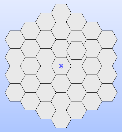
Fig. 13 Hexagonal lattice built by applying the three methods for adding cells.

Applying lattice’s type-specific symmetries

In addition to the common symmetry types that can be applied to a generic layout (see Applying a symmetry section), the CartesianLattice and the HexLattice classes supports the same symmetry types of the CartesianCell and HexCell classes respectively, as based on the same characteristic shape. See Applying cell’s type-specific symmetries for the supported types.

Independently from the lattice type, the result is the construction of a 2D shape used to derive the Region objects in common with the shape of the symmetry. For more details, please refer to the Applying a symmetry section.

Fig. 14 shows the results of applying a SIXTH symmetry to a hexagonal lattice.

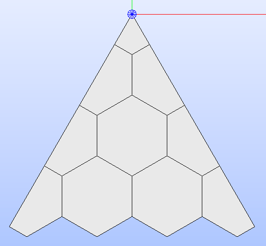
Fig. 14 Hexagonal lattice after applying the SIXTH type of symmetry.

Layout Export

The aim of GLOW is to provide DRAGON5 users with a tool that allows them to create geometry layouts not available natively and export the surface geometry representation to an output .dat file having a format similar to the one used by the APOLLO2 TDT solver. The .dat file can be used directly as input to the DRAGON5 SALT: module for producing tracking information in the DRAGON5 format. To meet this requirement, GLOW comes with a functionality for extracting the necessary information about the geometry and generate the output file in the required format.

Once the geometry layout has been created, users can run the export process by calling the function export_layout_to_tdt(). This function first analyses the provided instance of the Fillable subclasses to extract information about the characteristics of its geometry and the properties associated to its regions. A TDT file, whose name is provided as second parameter, is generated, collecting all this information.

Users can indicate which information about the geometry needs to be extracted from the layout and the tracking setup on the basis of specific configuration options defined in the dataclass TdtSetup, whose instance is provided to the export_layout_to_tdt() function. The available settings are the following ones:

• the geometry type of the layout (either the technological or the sectorised geometry), as item of the enumeration GeometryType. A value different from the one used to display the layout in the SALOME 3D viewer can be specified.

• the type of properties, as elements of the PropertyType enumeration, associated to the regions of the layout that should be included in the .dat file.

• the value for the albedo applied to the BCs of the layout. This information indicates how much reflective the BCs are, i.e. the ratio of exiting to entering neutrons. This attribute can assume values between 0.0 (no reflection) and 1.0 (full reflection), with the latter case indicating the ALBE 1.0 BC used in DRAGON5 with a uniform tracking (i.e. with the ISOTROPIC). If not specified, the default value corresponding to the layout type is adopted, i.e. 1.0 for the ISOTROPIC case and 0.0 for the other types.

• the value for the typgeo index of the .dat file. This value identifies the type of layout (in terms of symmetry and BCs) and of tracking (i.e. TSPC or TISO) to apply. Values are expressed in terms of elements of the LayoutGeometryType enumeration, and they match the ones expected by the SALT: module of DRAGON5.

• the type of symmetry to consider, as element of the enumeration SymmetryType. The indicated symmetry type is applied, if the corresponding shape of the symmetry has already been built by calling the apply_symmetry() method.

The function export_layout_to_tdt() also supports the possibility to export the surface geometry representation for a custom portion of the provided Fillable instance. This portion, which is GEOM compound, is provided as last argument to the export function. When providing a portion of the layout, users should note that the configuration values provided in the TdtSetup instance must match with the indicated GEOM compound object. If values that do not match with the shape of the compound are provided, the validity of the results in DRAGON5 cannot be assured.

The analysis step involves the extraction of the geometric data, that is needed for the generation of the output TDT file, from the layout. The first step consists in determining the Region objects that correspond to the GEOM faces the layout to export can be subdivided into. A traslation of layout, and of its regions, is performed, if needed, so that its lower-left corner coincides with the origin of the XYZ space as this is needed by DRAGON5 when processing the geometry layout with the SALT: module. In addition, if the SECTORIZED geometry type is indicated, the Region objects are partitioned according to the edges of the refined geometry.

For each Region object, a FaceData object is built and associated with the property types (PropertyType) for which the layout is analysed. In addition, an index is assigned to ensure their identification. For each GEOM edge object of the layout to export, an EdgeData instance is built storing the FaceData objects of the regions that share it. This means that each edge, identified with another index, has one or two regions associated with it. Edges that are shared by two adjacent regions are internal edges, while those associated with only one region are border edges.

Lastly, glow.generator.export_data.BoundaryData instances are built for each border of the layout to export. These instances store the indices of the corresponding border edges, as well as the type of boundary (as item of the BoundaryType enumeration) and its geometric data, both determined on the basis of the indicated LayoutGeometryType and the applied SymmetryType.

Table 1 provides the association between LayoutGeometryType and BoundaryType for the hexagonal and Cartesian type of layouts identified by the corresponding cell and lattice classes. In case of generic cells and lattices, all the LayoutGeometryType values are valid. The first group of columns LayoutGeometryType-BoundaryType indicates the values for which a uniform tracking (i.e. TISO) should be performed in SALT:; the second group refers to values which correspond to a cyclic tracking (i.e. TSPC). An ISOTROPIC type does not correspond to any BC, whereas those values that show two types of BCs correspond to a geometry layout in which a ROTATION is applied on the internal boundaries and a TRANSLATION on the external ones (see Fig. 15).

Table 1 Available combinations for TISO and TSPC cases.

LayoutType	SymmetryType	LayoutGeometryType	BoundaryType	LayoutGeometryType	BoundaryType
HEX	FULL	ISOTROPIC	/	HEXAGON_TRAN	TRANSLATION
	THIRD	ROTATION	TRANSLATION/ROTATION	R120	TRANSLATION/ROTATION
	SIXTH	SYMMETRIES_TWO	AXIAL_SYMMETRY	SA60	AXIAL_SYMMETRY
		ROTATION	TRANSLATION/ROTATION	RA60	TRANSLATION/ROTATION
	TWELFTH	SYMMETRIES_TWO	AXIAL_SYMMETRY	S30	AXIAL_SYMMETRY
RECT	FULL	ISOTROPIC	/	RECTANGLE_TRAN	TRANSLATION
				RECTANGLE_SYM	AXIAL_SYMMETRY
	HALF	SYMMETRIES_TWO	AXIAL_SYMMETRY	RECTANGLE_SYM	AXIAL_SYMMETRY
	DIAG	SYMMETRIES_TWO	AXIAL_SYMMETRY	RECTANGLE_EIGHTH	AXIAL_SYMMETRY
	QUARTER	SYMMETRIES_TWO	AXIAL_SYMMETRY	RECTANGLE_SYM	AXIAL_SYMMETRY
	EIGHTH	SYMMETRIES_TWO	AXIAL_SYMMETRY	RECTANGLE_EIGHTH	AXIAL_SYMMETRY

The items of the enumeration LayoutGeometryType identify the different values for the typgeo index in the .dat output file. The SALT: module of DRAGON5 associates one of the two types of tracking according to the typgeo value [3]:

• values of 0, 1 and 2 are associated with a TISO tracking type, which produces non-cycling tracks distributed uniformally over the domain.

• values greater that 2 are associated with a TSPC tracking type, which indicates a cyclic tracking over a closed domain.

The meaning of each items of the enumeration LayoutGeometryType is detailed in the following:

• ISOTROPIC to represent a layout having an isotropic reflection on its boundaries. It is associated with a TISO tracking.

• SYMMETRIES_TWO to represent a layout having symmetries of two axis of angle pi/n ( \(n>0\)) on its boundaries. It is associated with a TISO tracking.

• ROTATION to represent a layout with a rotation of angle 2*pi/n (\(n>1\)) for its boundaries. It is associated with a TISO tracking.

• RECTANGLE_TRAN to represent a Cartesian layout having a translation BC on its boundaries. It is associated with a TSPC tracking.

• RECTANGLE_SYM to represent a full, half, or quarter symmetry for a Cartesian layout. It is associated with a TSPC tracking.

• RECTANGLE_EIGHT to represent a layout with an eighth symmetry. It is associated with a TSPC tracking.

• SA60 to represent a layout with a sixth symmetry. It is associated with a TSPC tracking.

• HEXAGON_TRAN to represent a full hexagonal layout having a translation BC on its boundaries. It is associated with a TSPC tracking.

• RA60 to represent a layout with a sixth symmetry with both rotation and translation BCs on its boundaries. It is associated with a TSPC tracking.

• R120 to represent a layout with an third symmetry with both rotation and translation BCs on its boundaries. It is associated with a TSPC tracking.

• S30 to represent a layout with a twelfth symmetry. It is associated with a TSPC tracking.

The different values of BCs that are automatically applied by GLOW to the boundaries of the geometry layout to export are identified by the items of the enumeration BoundaryType. Their meaning and usage is the same as specified in [3]:

• VOID, indicating that boundaries have zero re-entrant angular flux;

• REFL, indicating a reflective boundary condition;

• TRANSLATION, indicating that the analysed layout is connected to another one for all its boundaries, thus treating an infinite geometry with translation symmetry;

• ROTATION, indicating a rotation symmetry;

• AXIAL_SYMMETRY, indicating a reflection symmetry;

• CENTRAL_SYMMETRY, indicating a mirror reflective boundary condition.

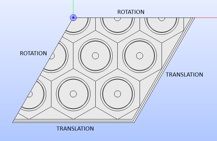
Fig. 15 Showing to which borders the ROTATION and TRANSLATION BC types are assigned to (THIRD symmetry case).

Given all the geometric data extracted from the layout, the output file is generated. Its structure consists of five sections, that are:

• the header section, providing information about the type of geometry (typgeo value), the number of folds (nbfold value), which is consistent with the typgeo, the number of nodes (i.e. the regions), the number of elements (i.e. the edges).

• the regions section, providing a list of indices attributed to the regions in the lattice. It also contains the definition of the macros to indicate subvolumes of the assembly. Names and indices of the macros match the assignment of the corresponding MACRO type of property to the regions.

• the edges section, providing the geometric information about all the edges in the geometry layout, as well as the indices of the regions they belong to.

• the boundary conditions section, providing information about the BC types and the indices of the edges belonging to each boundary.

• the material section, indicating the index of each value of the MATERIAL type of property. The order in which values are present matches the indices of the regions.

Usage

GLOW can be used directly by writing down a Python script where the single needed modules can be imported; alternatively, users can import all the modules at once to have them available by setting the following import instruction:

from glow import *

Given that, classes and methods are directly accessible and users can exploit them to:

• assemble the geometry layout;

• assign properties to regions;

• visualise the result in the SALOME 3D viewer;

• export the geometry layout to a .dat file in the TDT-compatible format.

To run this script, users can:

• provide it as argument when running SALOME;

  salome my_script.py
  

• load it directly from within the SALOME application.

In addition, since SALOME comes with an embedded Python console, users can import the GLOW modules and exploit its functionalities directly.

The built script can also be executed in batch mode, i.e. without running the SALOME GUI, by providing it as argument when running SALOME shell environment:

salome shell my_script.py

To see some of the GLOW functionalities in action, please refer to the script files present in the tutorials folder and described in the Tutorials section. These examples are intended to show a few case studies and how they are managed in GLOW. For further information about the available classes and methods, please refer to the API guide section.