Tutorials

To fully exploit the functionalities offered by GLOW, several examples are provided. They can be found in the tutorials folder. In the following, they are presented and explained in detail, showing for each the resulting geometry layout as displayed in the 3D viewer of SALOME.

Hexagonal Cell

The use case hexagonal_cell.py shows the steps required to declare a single hexagonal cell and customise its geometry layout.

The goal is to instantiate a hexagonal cell whose edge is 1.0 long, having three circles to delimit the different regions where each one is attributed to a specific material. The cell’s technological geometry is built from a hexagonal cell with specified material, onto which several circular Region objects are added. Each Region object is added to a layer in the cell’s hierarchical structure. The order of insertions of the regions is from the outer to the inner region; this allows for the correct overlapping of regions one onto the other. Materials are assigned as values of the corresponding property type MATERIAL directly when instantiating the circular regions. The following code snippet shows the building steps:

# Intialise two lists, one storing the circular regions radii, the other
# the names of the materials, sorted from the inner to the outer region
radii = [0.25, 0.4, 0.6]
materials = ["MAT_1", "MAT_2", "MAT_3"]
# Build the cell's geometry layout by adding three circular regions from
# the outer to the inner
cell = HexCell(
    name="Hexagonal cell", base_props={PropertyType.MATERIAL: "MAT_4"}
)
for radius, mat in zip(radii[::-1], materials[::-1]):
    cell.add(
        Region(
            Circle(radius=radius),
            properties={PropertyType.MATERIAL: mat}
        )
    )

# Show the regions according to the 'MATERIAL' colour map
cell.show(PropertyType.MATERIAL)

The regions of the cell’s technological geometry can be displayed in the SALOME 3D viewer with the MATERIAL color map by specifying it among the available arguments of the method show(). The result is shown in Fig. 16.

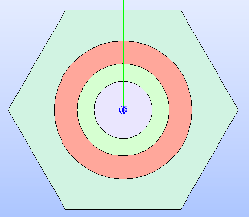
Fig. 16 Hexagonal cell’s technological geometry shown by applying a color map that highlights the type of property MATERIAL applied to the different regions.

Having a refined geometry layout can allow for capturing flux gradients arising from geometric heterogeneities. Hence, a sectorisation can be applied with the method sectorize(). It requires two lists, one with the number of sectors that each region is subdivided into and one with the angle that each sectorisation starts from. The refined geometry can be shown even with the MATERIAL colorset by specifying it among the arguments of the method show() together with the SECTORIZED type of geometry (see Fig. 17).

# Build the cell's sectorised geometry
cell.sectorize([1, 1, 6, 6], [0]*4)
# Show the cell's sectorised layout according to the 'MATERIAL' colour map
cell.show(PropertyType.MATERIAL, GeometryType.SECTORIZED)

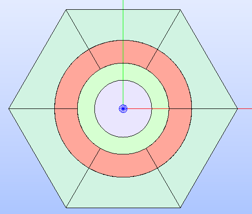
Fig. 17 Hexagonal cell’s sectorised geometry shown by applying a colour map that highlights the MATERIAL property type applied to the different regions.

Cartesian Cell With Custom Refined Layout

The use case cartesian_cell.py shows the steps required to declare a single Cartesian cell and customize its sectorised layout by means of the functions of the module glow.interface.geom_interface that wrap the ones of the GEOM module of SALOME.

The goal is to instantiate a Cartesian cell with a square shape whose edge is 1.0 long. The cell is subdivided into four regions by means of three circles; a specific material is assigned to each of the regions of the resulting technological geometry. The characterization of the cell’s technological geometry follows the same instructions as shown in the previous case with the instantiation of Region objects, each with a value for the MATERIAL property type.

# Intialise two lists, one storing the circular regions radii, the other
# the names of the materials, sorted from the inner to the outer region
radii = [0.2, 0.3, 0.4]
materials = ["MAT_1", "MAT_2", "MAT_3"]
# Build the cell's geometry layout by adding three circular regions from
# theouter to the inner
cell = CartesianCell(
    name="Cartesian cell", base_props={PropertyType.MATERIAL: "MAT_4"}
)
for radius, mat in zip(radii[::-1], materials[::-1]):
    cell.add(
        Region(
            Circle(radius=radius),
            properties={PropertyType.MATERIAL: mat}
        )
    )

To refine the geometry layout, a sectorisation can be applied with the method sectorize(). In addition to the two lists indicating the number of sectors and the angle the sectorisation starts from, a Cartesian cell can also receive the boolean flag windmill. This last option generates a sectorised geometry where lines are drawn between two adjacent border edges from points of intersection of the sector edges with the cell’s borders (see Fig. 18).

# Build the cell's sectorised geometry with 'windimill' option enabled
cell.sectorize([1, 1, 4, 8], [0, 0, 0, 22.5], windmill=True)
# Show the sectorised cell with regions colored according to the 'MATERIAL'
# property
cell.show(PropertyType.MATERIAL, GeometryType.SECTORIZED)

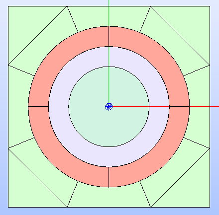
Fig. 18 Cartesian cell’s refined geometry with windmill sectorisation enabled. It is shown according to the MATERIAL colour map.

The method sectorize() only covers the subdivision of the technological geometry into sectors by drawing edges that are stored in the geometry_maps attribute of the subclass Fillable. If a further customisation is needed, users can rely on the functions in the glow.interface.geom_interface module to build the GEOM compound of edges that further refines the geometry layout. This tutorial demonstrates how to customise the cell by updating the sectorised geometry with a GEOM compound containing more circles between two adjacent regions of the technological geometry. By updating the GEOM compound that corresponds to the SECTORIZED geometry type, it is possible to have a custom refined layout. The result of the following code is shown in Fig. 19.

# Build a compound from the edges of the circles
circles_cmpd = make_compound([c.borders[0] for c in circles])
# Update the cell's sectorised geometry with the compound of edges
cell.geometry_maps[GeometryType.SECTORIZED] = wrap_shape(
    make_compound(
        [cell.geometry_maps[GeometryType.SECTORIZED], circles_cmpd]
    )
)
# Show the result in the 3D viewer
cell.show(PropertyType.MATERIAL, GeometryType.SECTORIZED)

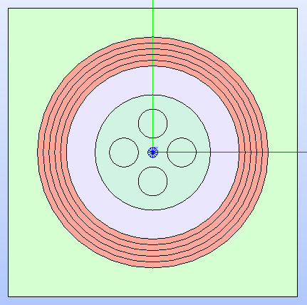
Fig. 19 Cartesian cell’s sectorised geometry after updating it by adding several circles. It is shown by applying a colour map that highlights the type of property MATERIAL.

Cartesian Assembly With Symmetry

The use case cartesian_assembly.py shows the steps required to declare an assembly made by a central cell (of Cartesian type) around which several rings of the same cell are placed. This type of geometry layout can be tracked by the SALT module of DRAGON5 using a one eighth symmetry as this is the minimum portion of the geometry that can describe the entire layout of the assembly.

The first step for assembling this use case geometry is to instantiate the Cartesian cell (i.e. object of the class CartesianCell) which constitutes the lattice. The instructions that follow build a Cartesian cell with a square shape whose edge is 1.0 long; the cell is subdivided into four regions by means of three circles and the type of property MATERIAL is assigned to each region. In addition, the regions are sectorised with the windmill option enabled.

# Intialise three lists one storing the circular regions radii, the other the
# names of the materials, sorted from the inner to the outer region
radii = [0.2, 0.3, 0.4]
materials = ["MAT_1", "MAT_2", "MAT_3"]
# Build the geometry layout of the cell by adding three circular regions, from
# external to internal
cell = CartesianCell(
    name="Cartesian cell", base_props={PropertyType.MATERIAL: "MAT_4"}
)
for radius, mat in zip(radii[::-1], materials[::-1]):
    cell.add(
        Region(
            Circle(radius=radius),
            properties={PropertyType.MATERIAL: mat}
        )
    )
# Apply the cell's sectorisation
cell.sectorize([1, 1, 4, 8], [0, 0, 0, 22.5], windmill=True)

The subsequent step is to declare the instance of the class CartesianLattice and add the cells it is made of. A single cell is provided when instantiating the lattice; this cell is placed at the centre of the lattice since the cell and the lattice share the same coordinates for their centres. To add several rings of the same cell, the method add_rings_of_cells() is provided with the instance of the CartesianCell class, previously declared, and the number of rings to add. Optionally, the starting ring index can be specified as third argument (it defaults to 1). The lattice’s technological geometry resulting from assembling all the rings of cells is shown in Fig. 20.

# Build the lattice with several rings of the same Cartesian cell
lattice = CartesianLattice([cell], name='Cartesian Lattice')
lattice.add_rings_of_cells(cell, 4, 1)
lattice.show(PropertyType.MATERIAL)

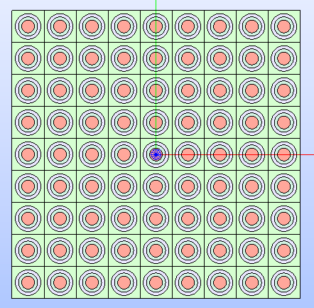
Fig. 20 Cartesian lattice’s technological geometry resulting by adding several rings of cells. It is shown by applying a colour map that highlights the type of property MATERIAL applied to the different regions of its cells.

To replicate a fuel assembly, the lattice needs to be framed into a box. This can be performed by declaring an additional CartesianCell instance and adding the lattice and the Region objects that represents the different box layers. Given the characteristic dimensions of the lattice, the width and the height of the cell is calculated and used to declare the assembly’s cell. To have the box cut the outmost ring of cells of the lattice, the rectangular inner region is built starting from the lattice dimensions reduced by a specific amount. The box contour can then be determined as the result of a cutting operation between the whole assembly and the inner region. Users should note that GLOW overloads mathematical operators to perform specific Boolean operations between subclasses of the GeomWrapper. In this case, the - operator is used to determine a new Region object from cutting the assembly with the inner region. Both the lattice and the box contour are added to the hierarchical tree of the assembly by calling the add() method. To simplify the hierarchical structure of a Fillable object, GLOW provides the method update_hierarchical_structure(). By default, this method collapses the layers of the layout by cutting those that are overlapped by superior layers. In addition, it can receive a Boolean flag that, if True, rebuilds the layers attribute with a list of one element that contains the Region objects belonging to the Fillable objects of the layout, thus reducing the hierarchical tree to one constituted only by the leaves (i.e. nodes are substituted by their leaves). Lastly, the method apply_symmetry() is called by specifying the EIGHTH type of symmetry. In the following, the instructions for assembling the assembly layout are detailed. The technological geometry resulting from assembling the box with the lattice is shown in Fig. 21.

# Build the cell representing the lattice's box so that it sligthly cuts
# the outmost ring of cells
assembly = CartesianCell(
    width_height=(box_w + 2*thickness, box_h + 2*thickness),
    base_props={PropertyType.MATERIAL: "MAT_2"}
)
# Build the inner region of the assembly that is cut out from the box shape
inner_area = Rectangle(
    height=(box_h - thickness),
    width=(box_w - thickness)
)
# Build the box contour as a 'Region' obtained by cutting the entire assembly
# with the inner region and assigning a material
box_contour = Region(
    assembly - inner_area,
    properties={PropertyType.MATERIAL: "MAT_2"}
)

# Add the lattice to the assembly cell, then apply the assembly layer region
assembly.add(lattice)
assembly.add(box_contour)

# Update the hierarchical tree of the layout and collapse all the layers into
# one, while cutting the refined geometry due to the box layer overlapping
# the outer cells
assembly.update_hierarchical_structure(True)
# Show the assembly technological layout with the property colour map
assembly.show(PropertyType.MATERIAL)

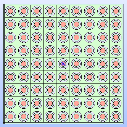
Fig. 21 Technological geometry layout of the assembly resulting by framing the cells in a box that sligthly cuts the outmost ring of cells.

A symmetry can be applied to the lattice’s geometry layout. For the specific layout of this use case, the EIGHTH type of symmetry can be used in tracking calculations since it is the minimum portion that can represent the entire geometry layout of the lattice. The result of applying the above mentioned type of symmetry is shown in Fig. 22.

# Apply the eighth symmetry type to the assembly
lattice.apply_symmetry(SymmetryType.EIGHTH)
# Show the resulting layout with the 'MATERIAL' colour map
lattice.show(PropertyType.MATERIAL)

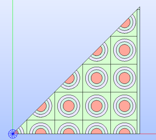
Fig. 22 Technological geometry layout of the assembly resulting by framing the lattice’s cells in a box and applying the EIGHTH type of symmetry.

If the SECTORIZED geometry type is specified when calling the show() method, the result is the technological layout with the edges resulting from the sectorisation of its cells. In case a further refinement is needed, users can rely on the specific functions of the glow.interface.geom_interface module that wrap the corresponding ones of the GEOM module of SALOME. In this tutorial, it is shown how to build a Cartesian mesh only for the box contour region. Given the characteristic dimensions of the lattice and the box layer thickness, two edges are built to represents the segments at the extrema of the mesh in the upper part of the box contour layer. Then, the subdivision edges of the mesh are built from the lattice’s pitch. A multi-translation of the built edge along the X-axis is performed so to build all the needed edges at once. A compound object collecting all the edges is built and rotated by 90° so that it is applied also to the right part of the box contour layer. The SECTORIZED geometry type of the assembly is then updated by applying a partition operation between the current compound stored in the geometry_maps attribute of the assembly and the compound collecting the mesh edges. The result is re-assigned to the same attribute and the assembly displayed according to the SECTORIZED geometry type with the MATERIAL colour map. The following code snippet presents the steps to build and display the assembly’s refined layout. The result is shown in :numref::assembly-refined.

# Get the X dimension of the pitch
pitch_x = cell.dimensions[0]
# Build XYZ axis vectors
o_x = make_vector((1, 0, 0))
o_y = make_vector((0, 1, 0))
o_z = make_vector((0, 0, 1))
# Build the outer edges of the mesh along Y by relying on the min/max lattice
# points
x_min, x_max, y_min, y_max = get_bounding_box(lattice.shape)
mesh_edge_outer_1 = make_edge(
    make_vertex((x_min + 0.5*thickness, y_min - thickness, 0.0)),
    make_vertex((x_min + 0.5*thickness, y_max + thickness, 0.0)),
)
mesh_edge_outer_2 = make_edge(
    make_vertex((x_max - 0.5*thickness, y_min - thickness, 0.0)),
    make_vertex((x_max - 0.5*thickness, y_max + thickness, 0.0)),
)
# Build the starting edges from which the Y-mesh is built with a 1D
# multi-translation
mesh_edge_1 = make_edge(
    make_vertex((x_min + pitch_x, y_min - thickness, 0.0)),
    make_vertex((x_min + pitch_x, y_max + thickness, 0.0)),
)
mesh_y = make_multi_translation_1d(mesh_edge_1, o_x, 1, 8)
# Join the Y-mesh edges into a single compound
mesh_y = make_compound([mesh_y, mesh_edge_outer_1, mesh_edge_outer_2])
# Rotate Y-mesh compound to obtain the X-mesh and join both in a compound
mesh_x = make_rotation(mesh_y, o_z, pi/2)
mesh = make_compound([mesh_x, mesh_y])

# Collect the refined geometry of the cells and join it with the built mesh
# by performing a partition
assembly.geometry_maps[GeometryType.SECTORIZED] = \
    assembly.get_geometry_map(GeometryType.SECTORIZED) // wrap_shape(mesh)

# Show the resulting refined layout with the 'MATERIAL' colour map
assembly.show(PropertyType.MATERIAL, GeometryType.SECTORIZED)

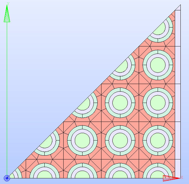
Fig. 23 One eighth of the assembly’s refined geometry layout resulting by joining the SECTORIZED edges of the cells with the mesh built for the box contour layer. Regions are displayed according to the MATERIAL colour map.

The geometry layout shown in :numref::assembly-refined can be exported to the output TDT file by calling the function export_layout_to_tdt(). It is possible to indicate which GeometryType to use in the analysis that GLOW performs to generate the output TDT file. In the following, the instance of the dataclass TdtSetup is provided specifying the SECTORIZED type of geometry, the adopted type_geo and the type of symmetry. The chosen value of type_geo allows for a TSPC type of tracking; the RECTANGLE_EIGHT value matches the applied symmetry type.

# Export the surface representation of the layout according to the TDT format
export_layout_to_tdt(
    assembly,
    "cartesian_assembly",
    TdtSetup(
        geom_type=GeometryType.SECTORIZED,
        type_geo=LayoutGeometryType.RECTANGLE_EIGHT,
        symmetry_type=SymmetryType.EIGHTH
    )
)

Hexagonal Assembly With Different Cells

The use case hexagonal_assembly.py shows the steps required to declare an assembly made by several rings of the same hexagonal cell framed in a hexagonal box. In addition, a hexagonal cell having different dimension, layout and materials is positioned at different XYZ coordinates within the lattice.

The first step to perform is creating the instances of the hexagonal cells (i.e. the object of the class HexCell) the lattice is made of. The two hexagonal cells are characterised by different length of their side edge as one is 1.0 and the other 2.0 long. The main pattern of the geometry layout is constituted by cells of the smaller size; they are subdivided into five regions by means of four circular regions. The cell with greater size, instead, has a different layout characterised by two circular regions. In addition, the first cell is rotated by 90° so that the final assembly is enclosed in a X-oriented hexagonal cell, as requested by the SALT module of DRAGON5 when dealing with a full layout. The type of property MATERIAL is assigned to the regions of each cell. The following snippet shows the instantiation of the two cells of the assembly. A dedicated function add_circular_regions() is included to handle the addition of the circular regions to the two cells.

def add_circular_regions(
        cell: Cell, radii: List[float], materials: List[float]
    ) -> None:
    """
    Function that adds cell-centred circular ``Region`` objects to the given
    ``Cell`` instance. Regions are characterised in terms of the radius and
    the material property.

    Parameters
    ----------
    cell : Cell
        The ``Cell`` instance the circular regions are added to.
    radii : List[float]
        The list of radii of the circular regions in ascending order.
    materials : List[str]
        The list of material names of the circular regions ordered from the
        inner to the outer region.
    """
    for radius, mat in zip(radii[::-1], materials[::-1]):
        cell.add(
            Region(
                Circle(radius=radius),
                properties={PropertyType.MATERIAL: mat}
            )
        )
# ----------------------------------------------------------------------
# Build the hexagonal cell that constitutes the lattice.
cell_1 = HexCell(
    name="Cell 1",
    base_props={PropertyType.MATERIAL: "COOLANT"}
)
cell_1.rotate(90)
add_circular_regions(
    cell_1, [0.1, 0.6, 0.625, 0.70], ["GAP", "FUEL", "GAP", "CLADDING"]
)

# ----------------------------------------------------------------------
# Build the second hexagonal cell
cell_2 = HexCell(
    side=2.0,
    name="Cell 2",
    base_props={PropertyType.MATERIAL: "COOLANT"}
)
add_circular_regions(cell_2, [1.0, 1.25], ['COOLANT', 'CLADDING'])

The subsequent step is to declare the instance of the class HexLattice and add the cells it is made of. A single cell (the one with smaller size) is provided when instantiating the lattice. This cell is placed at the centre of the lattice as they both have the same coordinates of the centre. Several rings of the same cell are then added with the method add_rings_of_cells(): the instance of the HexCell class, previously declared, is provided together with the number of rings to add, and the starting ring index. To complete the lattice’s geometry layout, the cell with greater size is added at specific coordinates using the method add(). The resulting geometry layout (see Fig. 24) shows that larger cells overlap smaller cells because they have been placed in a higher layer. Consequently, the layout of the cells being partially overlapped is automatically modified by the result of a cut operation. Cells that are completely overlapped, instead, are removed from the hierarchical tree of the lattice. The aforementioned operations are automatically performed by calling the show() method.

# Build the lattice and add both types of cells
lattice = HexLattice(cells=[cell_1], name="HexLattice")
lattice.add_rings_of_cells(cell_1, 6, 1)
# XY coordinates of the centres of the cells with greater size
x = 4.330127
y = 4.5
lattice.add(cell_2, ())
lattice.add(cell_2, (x, y, 0.0))
lattice.add(cell_2, (-x, y, 0.0))
lattice.add(cell_2, (x, -y, 0.0))
lattice.add(cell_2, (-x, -y, 0.0))
# Show the lattice's technological geometry with the 'MATERIAL' colour map
lattice.show(PropertyType.MATERIAL)

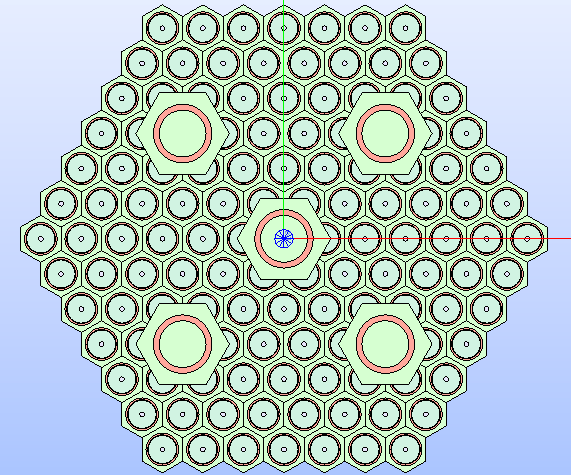
Fig. 24 Hexagonal lattice’s technological geometry resulting by adding several rings of cells with smaller size and cells with a greater size at specific coordinates. The resulting geometry layout shows that the cells of the higher layer cut those of the layer below. The colour map that highlights the type of property MATERIAL is applied to the different regions of the lattice’s cells.

The current lattice’s geometry layout shown in Fig. 24 presents a situation where the structural parts (e.g. regions associated with a fuel material) of the smaller cells are cut. Since this scenario cannot happen in real-life situations, these cells need to be restored by removing any circular region. The restore() method allows for resetting the cell’s geometry layout to its characteristic shape while clearing any associated properties. To get from within a Python script the cells to restore, this tutorial includes the function get_modified_cells(). Given the HexLattice instance, this function returns a list of cells of the lattice that show a geometry layout that differs from their characteristic shape. For each of the returned cells, the restore() method is called and then the MATERIAL property set to be COOLANT. Fig. 25 shows the result of restoring the cut cells.

def get_modified_cells(lattice: Lattice) -> List[Cell]:
    """
    Function that returns a list of ``Cell`` objects belonging to the given
    ``Lattice`` instance. These cells have their geometry layout changed
    compared to their original one.
    For each cell in each layer, the current shape of the cell is built and
    its area compared with the area of its specific characteristic figure (as
    a ``Surface`` instance).
    Those showing a different value for the area indicates a change in their
    geometry layout has occurred and are collected into the returned list.

    This function retrieves cells that have been modified within the lattice,
    such as by overlap with a superior layer of cells.

    Parameters
    ----------
    lattice : Lattice
        The lattice instance to check for cells whose geometry layout has
        changed.

    Returns
    -------
    List[Cell]
        A list of ``Cell`` objects whose geometry layout differs from their
        original one.
    """
    cells = []
    lattice.update_hierarchical_structure()
    for layer in lattice.layers:
        for layout in layer:
            if isinstance(layout, Region):
                continue
            # Build a face object over the borders of the cell
            cell_shape = make_face(build_compound_borders(layout))
            # Compare the area of the current cell's face with the one of its
            # original shape
            if not math.isclose(
                get_basic_properties(cell_shape)[1],
                get_basic_properties(layout.shape)[1],
                abs_tol=1e-6
            ):
                cells.append(layout)
    # Return the list of changed cells
    return cells

# Get the cells whose geometry layout has been cut and restore them by
# assigning a specific property type
for cell in get_modified_cells(lattice):
    cell.restore()
    cell.regions[0].properties = {PropertyType.MATERIAL: 'COOLANT'}

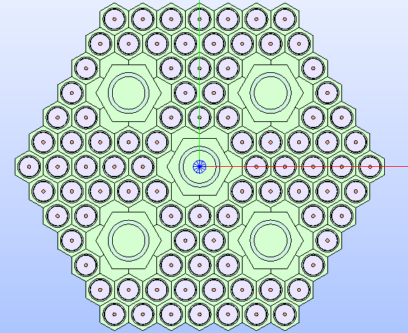
Fig. 25 Hexagonal lattice’s technological geometry resulting by restoring the geometry layout of those cells that have been cut. The colour map that highlights the type of property MATERIAL is applied to the different regions of the lattice’s cells.

An assembly requires the lattice to be included in the hierarchical tree of a cell, which represents the box. A HexCell object is then instantiated by specifying, as the size of its edge, the length of the side edge of the hexagon that encloses the lattice plus the sum of the thicknesses of the box layers. In this case, the box layers do not cut the outmost ring of cells, then, the layout can be built by adding the two box layers first (defined as Region instances), followed by the HexLattice instance. The resulting assembly is shown in Fig. 26.

# Build the assembly cell from the lattice's dimensions + the sum of the box's
# layers thickness
box_thicknesses = [0.15, 0.15]
assembly = HexCell(
    side=lattice.dimensions[0] + sum(box_thicknesses),
    name="Hexagonal Assembly",
    base_props={PropertyType.MATERIAL: 'COOLANT'}
)
# Add the box layers first, then the lattice
assembly.add(
    Region(
        Hexagon(edge_length=lattice.dimensions[0]+box_thicknesses[0]),
        properties={PropertyType.MATERIAL: 'CLADDING'}
    )
)
assembly.add(
    Region(
        Hexagon(edge_length=lattice.dimensions[0]),
        properties={PropertyType.MATERIAL: 'COOLANT'}
    )
)
assembly.add(lattice)
# Show the lattice's technological geometry
assembly.show(PropertyType.MATERIAL)

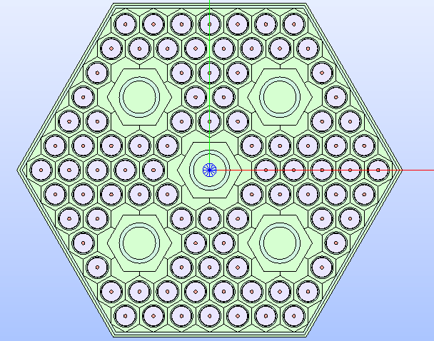
Fig. 26 Hexagonal lattice’s technological geometry resulting by framing the lattice into a hexagonal cell.

The geometry layout shown in Fig. 26 can be exported to the output TDT file by calling the function export_layout_to_tdt(). In this case, the layout is exported by indicating, in the TdtSetup dataclass, a value of type_geo that results in a TRANSLATION BC type applied to the lattice’s boundaries. No values for the GeometryType and the SymmetryType are provided; this means that the default TECHNOLOGICAL and FULL values are considered. The adopted value of type_geo results in a TRANSLATION BC type applied to the lattice’s boundaries. This setting generates a surface representation that must be tracked by a cyclic method (i.e. TSPC).

# ----------------------------------------------------------------------
# Perform the geometry analysis and export the TDT file of the surface
# geometry
export_layout_to_tdt(
    assembly,
    'hexagonal_assembly',
    TdtSetup(type_geo=LayoutGeometryType.HEXAGON_TRAN)
)

Colorset

The use case colorset.py shows the steps required to build the S30 portion of a colorset made by two different hexagonal assemblies. The layout of the colorset presents a control rod assembly surrounded by six fuel assemblies. In the specific case of this example, given the available symmetry of one twelfth of the colorset (i.e. S30), only the two assemblies that concur in identifying the portion to study are built.

The first step in assembling the geometry layout is building the fuel assembly, which is made by two hexagonal cells (i.e. the object of the class HexCell) with different layouts.

The two hexagonal cells that characterise the lattice are built with the same edge of 1.0, but different number of circular regions. The cell which constitutes the main pattern of the geometry layout is subdivided into five regions by means of four circles; the other cell, which is placed in the lattice centre, is characterized by two circular regions. In addition, both cells are rotated by 90° so that the final assembly is enclosed in a X-oriented hexagonal cell. The type of property MATERIAL is assigned to the regions of each cell. A dedicated function add_circular_regions() is included to handle the addition of the circular regions to the two cells.

def add_circular_regions(
        cell: Cell, radii: List[float], materials: List[float]
    ) -> None:
    """
    Function that adds cell-centred circular ``Region`` objects to the given
    ``Cell`` instance. Regions are characterised in terms of the radius and
    the material property.

    Parameters
    ----------
    cell : Cell
        The ``Cell`` instance the circular regions are added to.
    radii : List[float]
        The list of radii of the circular regions in ascending order.
    materials : List[str]
        The list of material names of the circular regions ordered from the
        inner to the outer region.
    """
    for radius, mat in zip(radii[::-1], materials[::-1]):
        cell.add(
            Region(
                Circle(radius=radius),
                properties={PropertyType.MATERIAL: mat}
            )
        )

# -------------------------------------------------------------------------- #
# FUEL ASSEMBLY CONSTRUCTION                                                 #
# -------------------------------------------------------------------------- #
# Build the hexagonal cells of the fuel assembly
fuel_cell = HexCell(
    name="Fuel cell", base_props={PropertyType.MATERIAL: "COOLANT"}
)
fuel_cell.rotate(90)
# Add the circular regions with their materials
add_circular_regions(
    fuel_cell, [0.2, 0.6, 0.62, 0.68], ["GAP", "FUEL", "GAP", "CLADDING"]
)

central_cell = HexCell(
    name="Central cell", base_props={PropertyType.MATERIAL: "COOLANT"}
)
central_cell.rotate(90)
add_circular_regions(central_cell, [0.6, 0.65], ["GAP", "CLADDING"])

The fuel assembly is built by instantianting an object of the class HexLattice and adding the cells it is made of. The central cell, which does not contain fuel material, is provided when instantiating the lattice. Several rings of the same fuel cell are then added with the method add_rings_of_cells(): the instance of the HexCell class, previously declared, is provided together with the number of rings to add. To complete the fuel assembly’s geometry layout, a new HexCell instance is created. The length of its edge derives from the one of the characteristic shape of the lattice plus the sum of all the thicknesses of the layers of the box cell. The layer identifying the cladding is built as a Region object resulting from cutting the Hexagon that corresponds to the region of cladding with another hexagon. Both the lattice and the cladding layer region are added to the fuel assembly cell resulting in the cells of the outmost ring to be cut by the box layer. The resulting assembly is shown in Fig. 27.

# -------------------------------------------------------------------------- #
# FUEL ASSEMBLY CONSTRUCTION                                                 #
# -------------------------------------------------------------------------- #
# Build the fuel assembly lattice of the colorset
fuel_lattice = HexLattice([central_cell], name="Fuel Assembly Lattice")
fuel_lattice.add_rings_of_cells(fuel_cell, 5)
# Build the cell framing the fuel lattice into a fuel assembly and add regions
# for layers and the lattice
layers_t = [-0.1, 0.3, 0.3]
fuel_assembly = HexCell(
    side=fuel_lattice.dimensions[0] + sum(layers_t),
    base_props={PropertyType.MATERIAL: "COOLANT"}
)
cladding_layer = Region(
    Hexagon(edge_length=fuel_lattice.dimensions[0] + layers_t[1])
    - Hexagon(edge_length=fuel_lattice.dimensions[0] + layers_t[0]),
    properties={PropertyType.MATERIAL: "CLADDING"}
)
fuel_assembly.add(fuel_lattice)
fuel_assembly.add(cladding_layer)

# Display the fuel assembly with the MATERIAL colour map
fuel_assembly.show(PropertyType.MATERIAL)

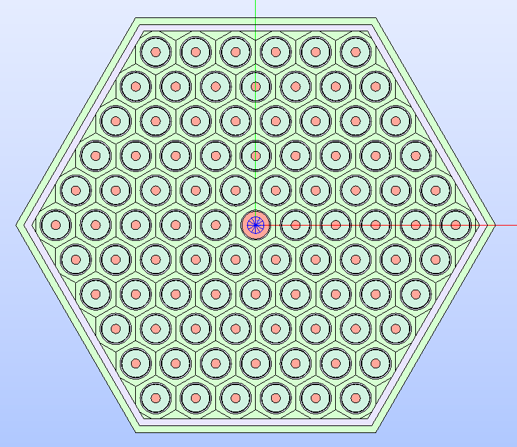
Fig. 27 The fuel assembly’s technological geometry resulting by framing the lattice into a box cell. Regions are displayed according to the MATERIAL colour map.

The second step in deriving the colorset layout is building the control rod assembly. Its layout is characterised by control rod pins, modelled as circles, placed within a central circular area. A HexCell object is adopted to replicate the layout of the control rod assembly. Region objects are created to replicate the box layers (using hexagonal shapes), the cell-centred circular regions, as well as the layout of the control rods (made by overlapping circular regions).

# -------------------------------------------------------------------------- #
# CONTROL ROD ASSEMBLY CONSTRUCTION                                          #
# -------------------------------------------------------------------------- #
# Data
pitch = fuel_assembly.dimensions[1] * 2
edge_bypass = (pitch) / math.sqrt(3)
edge_ext_wrap_o = (pitch - 0.4) / math.sqrt(3)
edge_ext_wrap_i = (pitch - 0.6) / math.sqrt(3)
r_cr_circles_i = 3.2
r_cr_circles_o = 5.2
cr_pin_radii = [0.68, 0.7, 0.78]
cr_wrapper_radii = [7, 7.25]
int_shaft_ir = 1.4
int_shaft_or = 1.7

# Build the control rod assembly as a hexagonal cell
cr_assembly = HexCell(
    side=edge_bypass,
    name= "Control Rod Assembly",
    base_props={PropertyType.MATERIAL: "COOLANT"}
)
# Add the box layers
cr_assembly.add(
    Region(
        Hexagon(edge_length=edge_ext_wrap_o),
        properties={PropertyType.MATERIAL: "CR_CLADDING"}
    )
)
cr_assembly.add(
    Region(
        Hexagon(edge_length=edge_ext_wrap_i),
        properties={PropertyType.MATERIAL: "CR_MIX"}
    )
)

# Add the circles representing the different zones of the wrapper
add_circular_regions(
    cr_assembly, cr_wrapper_radii, ["COOLANT", "CR_CLADDING"]
)

To build and properly position the control rod pins, the create_vertices_list function is included in the script: it produces a list with a given number of vertex objects laying on the same circumference with the given radius. For each calculated vertex, the three Region objects that characterise the control rod layout are built and added to the assembly. To reduce the tree complexity, the same layer index is indicated when calling the add() method. If not provided, each regions would have been added to a new layer.

def create_vertices_list(circle_radius: float, n_vertices: int) -> List[Any]:
    """
    Function that creates a list of vertex objects laying on the same
    circumference with the given radius. The number of vertices is provided
    as input.

    Parameters
    ----------
    circle_radius : float
        The radius of the circle on whose circumference the vertices are
        placed.
    n_vertices : int
        The number of vertices to build.

    Returns
    -------
    List[Any]
        The list of vertex objects laying on the same circumference.
    """
    # Build the circle
    circle = Circle(
        radius=circle_radius, name=f"Circle with radius {circle_radius}")
    vertices = []
    # Build the vertices on the circle's circumference
    for n in range(n_vertices):
        vertex = make_vertex_on_curve(circle.borders[0], n/n_vertices)
        vertices.append(vertex)
    return vertices

# Build the vertices at which the control rod regions are placed
cr_vertices_i = create_vertices_list(r_cr_circles_i, 6)
cr_vertices_o = create_vertices_list(r_cr_circles_o, 12)
# Build the circular control rod regions placed along two circumferences by
# specifying the same layer index (the last one) to reduce tree complexity
for v in cr_vertices_i + cr_vertices_o:
    cr_assembly.add(
        Region(
            Circle(radius=cr_pin_radii[2]),
            properties={PropertyType.MATERIAL: "CR_CLADDING2"}
        ),
        get_point_coordinates(v),
        len(cr_assembly.layers)
    )
    cr_assembly.add(
        Region(
            Circle(radius=cr_pin_radii[1]),
            properties={PropertyType.MATERIAL: "GAP"}
        ),
        get_point_coordinates(v),
        len(cr_assembly.layers)
    )
    cr_assembly.add(
        Region(
            Circle(radius=cr_pin_radii[0]),
            properties={PropertyType.MATERIAL: "ABSORBER"}
        ),
        get_point_coordinates(v),
        len(cr_assembly.layers)
    )

Lastly, the layout of the shaft is built; this is represented by two overlapping circular regions added with the provided add_circular_regions function. The resulting layout is shown in Fig. 28.

# Build the central shaft as made by two overlapping circular regions
add_circular_regions(
    cr_assembly, [int_shaft_ir, int_shaft_or], ["COOLANT", "CR_CLADDING"]
)
# Display the control rod assembly
cr_assembly.show(PropertyType.MATERIAL)

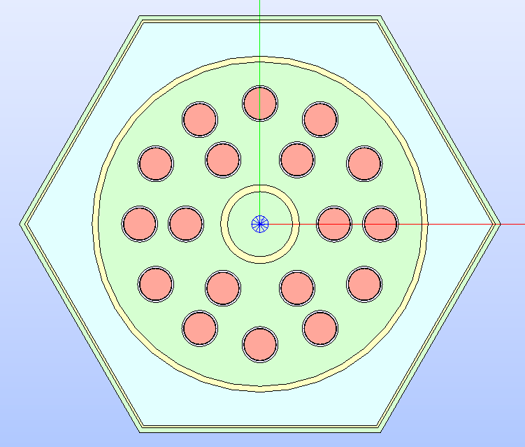
Fig. 28 The control rod assembly’s technological geometry whose regions are displayed according to the MATERIAL colour map.

To replicate the layout of the colorset, either a HexLattice or a Lattice instance could be used. In this specific case, only two cells are needed and the Lattice class is used. The fuel assembly cell is translated to the right of the control rod assembly, which keeps its position in the XYZ origin. Both HexCell objects are provided to the Lattice class when it is instantiated. A custom one twelfth symmetry is adopted by building the corresponding GEOM face object and using it for extracting the layout to export. The latter operation requires a common operation between the entire layout and the shape of the symmetry. The corresponding make_common function is used. The resulting GEOM compound object of the colorset portion is added to the SALOME study with the add_to_study function.

# -------------------------------------------------------------------------- #
# COLORSET CONSTRUCTION                                                      #
# -------------------------------------------------------------------------- #
# Translate the fuel assembly to the right of the control rod assembly
fuel_assembly.translate(
    (3/2*cr_assembly.dimensions[0], cr_assembly.dimensions[1], 0)
)

# Build the colorset as a 'Lattice' with the two assembly cells
colorset = Lattice([cr_assembly, fuel_assembly], (0.0, 0.0, 0.0), "Colorset")
# Display the colorset
colorset.show(PropertyType.MATERIAL)

# -------------------------------------------------------------------------- #
# COLORSET S30 SYMMETRY CONSTRUCTION                                         #
# -------------------------------------------------------------------------- #
# Extract the S30 symmetry portion out of the entire colorset
edges = build_contiguous_edges(
    [
        make_vertex((0.0, 0.0, 0.0)),
        make_vertex((
            3/2*fuel_assembly.dimensions[0],
            fuel_assembly.dimensions[1],
            0.0
        )),
        make_vertex((2*fuel_assembly.dimensions[0], 0.0, 0.0))
    ]
)
cutting_face = make_face(edges)
colorset_portion = make_common(colorset, cutting_face)
add_to_study(colorset_portion, "Colorset - S30 Symmetry")

To enable the visualization of the regions of the colorset portion that belong to the two assemblies at once with the same MATERIAL colour map, dedicated functions are called. First, the Region objects that correspond to the GEOM faces the built compound is made of are extracted with the build_compound_regions() function. Then, a unique colour is associated to each region having the same material name by means of the associate_colors_to_regions() A loop through all the Region objects is performed: the GEOM face each region corresponds to is coloured with the set_color_face() and added to the SALOME study with the add_to_study_in_father() function so that each region is displayed as a children of the colorset compound. The result is show in Fig. 29.

# -------------------------------------------------------------------------- #
# COLORSET REGIONS VISUALIZATION                                             #
# -------------------------------------------------------------------------- #
# For each face in the colorset compound, recover the corresponding 'Region'
# in the colorset 'Lattice' and build the corresponding region to display
colorset_regions = build_compound_regions(colorset_portion, colorset.regions)
# Associate a unique colour to each region according to the material name
associate_colors_to_regions(PropertyType.MATERIAL, colorset_regions)
# Display the regions of the colorset portion with the material colour map
for region in colorset_regions:
    set_color_face(region, region.color)
    add_to_study_in_father(colorset_portion, region, region.name)

update_salome_study()

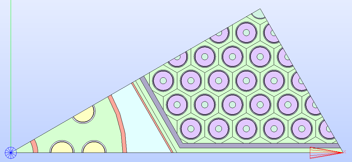
Fig. 29 The technological geometry of the colorset portion replicating the custom S30 symmetry. Its regions are displayed according to the MATERIAL colour map.

Lastly, the surface geometry representation of the colorset portion is exported to an output TDT file using the export_layout_to_tdt() function by providing the GEOM compound object of the colorset portion directly. The TdTSetup instance is configured so that the SALT module of DRAGON5 considers the exported layout to be one twelfth of the full layout to which isotropic tracking (TISO) must be applied.

# -------------------------------------------------------------------------- #
# COLORSET S30 PORTION TDT EXPORT                                            #
# -------------------------------------------------------------------------- #
# Generate the TDT file from the colorset portion using a specific typgeo and
# symmetry type
export_layout_to_tdt(
    colorset,
    "colorset_s30",
    tdt_setup=TdtSetup(
        type_geo=LayoutGeometryType.SYMMETRIES_TWO,
        symmetry_type=SymmetryType.TWELFTH
    ),
    compound_to_export=colorset_portion
)